User Guide

Preface

All of the documentation in this page, and elsewhere assumes you have imported the pyDeltaRCM package as pyDeltaRCM:

>>> import pyDeltaRCM

Additionally, the documentation frequently refers to the numpy and matplotlib packages. We may not always explicitly import these packages throughout the documentation; we may refer to these packages by their common shorthand as well.

>>> import numpy as np
>>> import matplotlib.pyplot as plt

Running the model

Running a pyDeltaRCM model is usually accomplished via a combination of configuration files and scripts. In the simplest case, actually, none of these are required; the following command (executed at a console) runs a pyDeltaRCM model with the default set of model parameters for 10 timesteps:

$ pyDeltaRCM --timesteps 10

Internally, this console command calls a Python function that runs the model via a method. Python code and scripts are the preferred and most common model use case. Let’s do the exact same thing (run a model for 10 timesteps), but do so with Python code.

Python is an object-oriented programming language, which means that the pyDeltaRCM model is set up to be manipulated as an object. In technical jargon, the pyDeltaRCM model is built out as a Python class, specifically, it is a class named DeltaModel; so, the actual model is created by instantiating (making an instance of a class) the DeltaModel. Python objects are instantiated by calling the class name, followed by parentheses (and potentially any input arguments), from a python script (or at the Python console):

>>> mdl = pyDeltaRCM.DeltaModel()

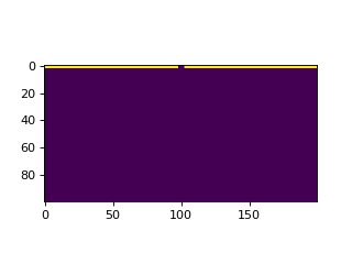
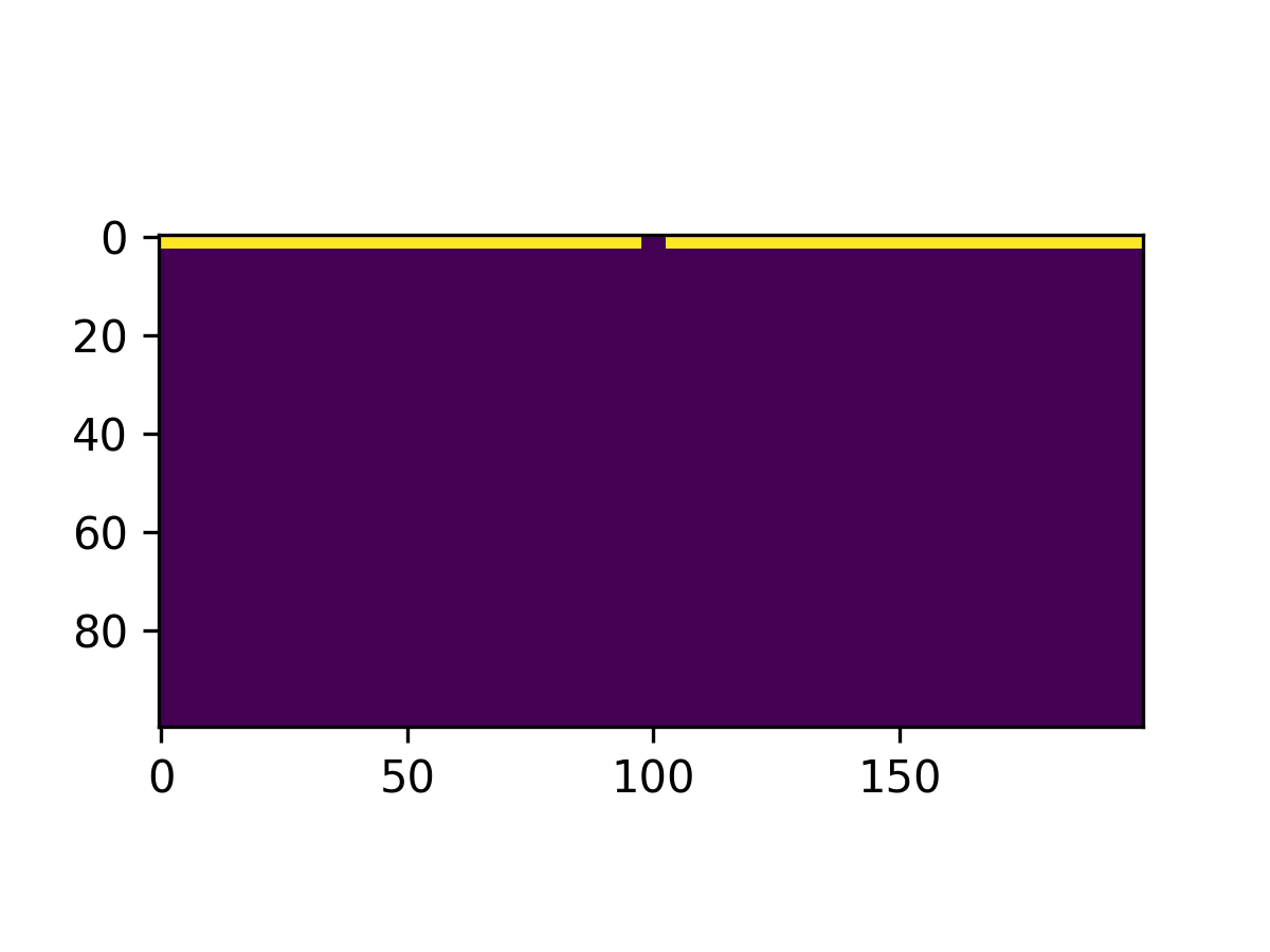
Here, mdl is an instance of the DeltaModel class; mdl is an actual model that we can run. Based on the default parameters, the model domain is configured as an open basin, with an inlet centered along one wall. Default parameters are set to sensible values, and generally follow those described in [1].

(png, hires.png)

To run the model, we use the update() method of the DeltaModel instance (i.e., call update() on mdl):

>>> for _ in range(0, 5):
...     mdl.update()

The update() method manages a single timestep of the model run. Check out the docstring of the method for a description of the routine, and additional steps that are called from update. Additionally, it may be helpful to read through the model informational guides.

Note

The model timestep (dt) is determined by model stability criteria; see the model stability guide for more information.

Finally, we need to tie up some loose ends when we are done running the model. We use the finalize method of the DeltaModel instance (i.e., call finalize() on mdl):

>>> mdl.finalize()

Specifically, calling finalize() will ensure that any data output during the model run to the output NetCDF4 file is correctly saved to the disk and does not become corrupted while the script is exiting. Note that the output file is periodically saved during the model run, so things might be okay if you forget to finalize() at the end of your simulation, but it is considered a best practice to explicitly close the output file with finalize().

Putting the above snippets together gives a complete minimum working example script:

>>> mdl = pyDeltaRCM.DeltaModel()

>>> for _ in range(0, 5):
...    mdl.update()

>>> mdl.finalize()

Now, we probably don’t want to just run the model with default parameters, so the remainder of the guide will cover other use cases with increasing complexity; first up is changing model parameter values via a YAML configuration file.

Configuring an input YAML file

The configuration for a pyDeltaRCM run is set up by a parameter set, usually described in the YAML markup format. To configure a run, you should create a file called, for example, model_configuration.yml. Inside this file you can specify parameters for your run, with each parameter on a new line. For example, if model_configuration.yml contained the line:

S0: 0.005
seed: 42

then a DeltaModel model instance initialized with this file specified as input_file will have a slope of 0.005, and will use a random seed of 42. Multiple parameters can be specified line by line.

Default values are substituted for any parameter not explicitly given in the input_file .yml file. Default values of the YAML configuration are listed in the Default Model Variable Values.

Important

The best practice for model configurations is to create a YAML file with only the settings you want to change specified. Hint: comment a line out with # so it will not be used in the model.

Hint

Check the model log files to make sure your configuration was interpreted as you expected!

Starting model runs

There are two API levels at which you can interact with the pyDeltaRCM model. There is a “high-level” model API, which takes as argument a YAML configuration file, and will compose a list of jobs as indicated in the YAML file; the setup can be configured to automatically execute the job list, as well. The “low-level” API consists of creating a model instance from a YAML configuration file and manually handling the timestepping, or optionally, augmenting operations of the model to implement new features. Generally, if you are modifying the model source code or doing anything non-standard with your simulation runs, you will want to use the low-level API. The high-level API is extremely helpful for exploring parameter spaces.

High-level model API

The high-level API is accessed via either a shell prompt or python script, and handles setting up the model configuration and running the model a specified duration.

For the following high-level API demonstrations, consider a YAML input file named model_configuration.yml which looks like:

S0: 0.005
seed: 42
timesteps: 500

Command line API

To invoke a model run from the command line using the YAML file model_configuration.yml defined above, we would simply call:

pyDeltaRCM --config model_configuration.yml

or equivalently:

python -m pyDeltaRCM --config model_configuration.yml

These invocations will run the pyDeltaRCM preprocessor with the parameters specified in the model_configuration.yml file. If the YAML configuration indicates multiple jobs (via matrix expansion or ensemble specification), the jobs will each be run automatically by calling update on the model 500 times.

Python API

The Python high-level API is accessed via the Preprocessor object. First, the Preprocessor is instantiated with a YAML configuration file (e.g., model_configuration.yml):

>>> pp = preprocessor.Preprocessor(p)

which returns an object containing the list of jobs to run. Jobs are then run with:

>>> pp.run_jobs()

Model simulation duration in the high-level API

The duration of a model run configured with the high-level API can be set up with a number of different configuration parameters.

Note

see the complete description of “time” in the model: Time in pyDeltaRCM.

Using the high-level API, you can specify the duration to run the model by two mechanisms: 1) the number of timesteps to run the model, or 2) the duration of time to run the model.

The former case is straightforward, insofar that the model determines the timestep duration and the high-level API simply iterates for the specified number of timestep iterations. To specify the number of timesteps to run the model, use the argument --timesteps at the command line (or timesteps: in the configuration YAML file, or timesteps= with the Python Preprocessor).

$ pyDeltaRCM --config model_configuration.yml --timesteps 5000

The second case is more complicated, because the time specification is converted to model time according to a set of additional parameters. In this case, the model run end condition is that the elapsed model time is equal to or greater than the specified input time. Importantly, this means that the duration of the model run is unlikely to exactly match the input condition, because the model timestep is unlikely to be a factor of the specified time. Again, refer to the complete description of model time Time in pyDeltaRCM for more information.

To specify the duration of time to run the model in seconds, simply use the argument --time at the command line (or time: in the configuration YAML file, or time= with the Python Preprocessor). It is also possible to specify the input run duration in units of years with the similarly named argument --time_years (time_years:, time_years=).

$ pyDeltaRCM --config model_configuration.yml --time 31557600
$ pyDeltaRCM --config model_configuration.yml --time_years 1

would each run a simulation for \((86400 * 365.25)\) seconds, or 1 year.

Important

Do not specify both time arguments, or specify time arguments with the timesteps argument. In the case of multiple argument specification, precedence is given in the order timesteps > time > time_years.

When specifying the time to run the simulation, an additional parameter determining the intermittency factor (\(I_f\)) may be specified --If at the command line (If: in the YAML configuration file, If= with the Python Preprocessor). This argument will scale the specified time-to-model-time, such that the scaled time is equal to the input argument time. Specifying the \(I_f\) value is essential when using the model duration run specifications. See Time in pyDeltaRCM for complete information on the scaling between model time and elapsed simulation time.

Running simulations in parallel

The high-level API provides the ability to run simulations in parallel on Linux environments. This option is only useful in the case where you are running multiple jobs with the matrix expansion, ensemble expansion, or set expansion tools.

To run jobs in parallel simply specify the –parallel flag to the command line interface. Optionally, you can specify the number of simulations to run at once by following the flag with a number.

$ pyDeltaRCM --config model_configuration.yml --timesteps 5000 --parallel
$ pyDeltaRCM --config model_configuration.yml --timesteps 5000 --parallel 6

Low-level model API

The low-level API is the same as that described at the beginning of this guide. Interact with the model by creating your own script, and manipulating model outputs at the desired level. The simplest case to use the low-level API is to do

>>> delta = pyDeltaRCM.DeltaModel(input_file='model_configuration.yml')

>>> for _ in range(0, 5000):
...    delta.update()

>>> delta.finalize()

However, you can also inspect/modify the update method, and change the order of operations, or add operations, as desired; see the guide to customizing the model below. If you are working with the low-level API, you can optionally pass any valid key in the YAML configuration file as a keyword argument during model instantiation. For example:

>>> delta = pyDeltaRCM.DeltaModel(input_file='model_configuration.yml',
...                    SLR=1e-9)

Keyword arguments supplied at this point will supersede values specified in the YAML configuration. See our guide for model customization for a complete explanation and demonstration for how to modify model behavior.

Advanced model configurations

Configuring multiple model runs from a single YAML file

Multiple model runs (referred to as “jobs”) can be configured by a single .yml configuration file and passing the file to the high-level API. Multiple runs can be configured by using the matrix, ensemble, and set configuration keys in the .yml file.

Important

You cannot use any of matrix ensemble or set with the low-level API. If you need, you could use the high-level API to generate the scripts for each job (e.g., timesteps: 0) and then manually generate DeltaModel instances from each .yml file to then use with the low-level API.

Matrix expansion

To use matrix expansion to configure multiple model runs, the dimensions of the matrix (i.e., the variables you want to run) should be listed below the matrix key. For example, the following configuration is a one-dimensional matrix with the variable f_bedload:

out_dir: 'out_dir'
dx: 40.0
h0: 1.0

matrix:
  f_bedload:
    - 0.5
    - 0.2

This configuration would produce two model runs, one with bedload fraction (f_bedload) 0.5 and another with bedload fraction 0.2, and both with grid spacing (dx) 2.0 and basin depth (h0) 1.0. The matrix expansions will create two folders at ./out_dir/job_000 and ./out_dir/job_001 that each correspond to a created job. Each folder will contain a copy of the configuration file used for that job; for example, the full configuration for job_000 is:

out_dir: 'out_dir/job_000'
dx: 40.0
h0: 1.0
f_bedload: 0.5

Additionally, a log file for each job is located in the output folder, and any output grid files or images specified by the input configuration will be located in the respective job output folder (note: there is no output NetCDF4 file for these runs).

Note

You must specify the out_dir key in the input YAML configuration to use matrix expansion.

Multiple dimensional matrix expansion is additionally supported. For example, the following configuration produces six jobs:

out_dir: 'out_dir'

matrix:
  f_bedload:
    - 0.5
    - 0.4
    - 0.2
  h0:
    - 1
    - 5

Ensemble expansion

Ensemble expansion creates replicates of specified model configurations with different random seed values. Like the matrix expansion, the out_dir key must be specified in the input configuration file. The ensemble key can be added to any configuration file that does not explicitly define the random seed. As an example, two model runs can be generated with the same input sediment fraction using the following configuration .yml:

out_dir: 'out_dir'

f_bedload: 0.5
ensemble: 2

This configuration file would produce two model runs that share the same parameters, but have different initial random seed values. The ensemble expansion can be applied to configuration files that include a matrix expansion as well:

out_dir: 'out_dir'

ensemble: 3

matrix:
  h0:
    - 1.0
    - 2.0

The above configuration file would produce 6 model runs, 3 with a basin depth (h0) of 1.0, and 3 with a basin depth of 2.0.

Hint

If you are debugging and experimenting, it may be helpful to comment out a line in your YAML, rather than deleting it completely! E.g., # ensemble: 3) would disable ensemble expansion.

Set expansion

Set expansion enables user-configured parameter sets to take advantage of the Preprocessor infrastructure (such as the job output preparation and ability to run jobs in parallel), while also enabling flexible configurations for parameter sets that cannot be configured via matrix expansion. For example, to vary Qw0 while holding Qs0 fixed requires modifying both C0_percent and some water-discharge-controlling parameter simultaneously; this cannot be achieved with matrix expansion.

To use set expansion, add the set key to a configuration file, and define a list of dictionaries which set the parameters of each run to be completed. For example, to configure two model runs, the first with parameters u0: 1.0 and h0: 1.0, and the second with parameters u0: 1.2 and h0: 1.2:

set:
  - {u0: 1.0, h0: 1.0}
  - {u0: 1.2, h0: 1.2}

All jobs in the set specification must have the exact same set of keys.

Note

Set expansion works with ensemble expansion, whereby each item in the set list is replicated ensemble number of times (with varied seed). Note that, matrix specification is not supported with the set specification.

Customizing model operations with subclasses and hooks

The DeltaModel is designed for flexibility and extension by users, and to support arbitrary and imaginative changes to the model routine. For example, one could easily extend the model to include additional delta controls (such as vegetation or permafrost development), or modify the model domain boundary conditions (such as imposing a sloped receiving basin). This flexibility is achieved by “subclassing” the DeltaModel to create a custom model object, and using “hooks” in the model to achieve the desired modifications.

Important

If you plan to customize the model, but did not follow the developer installation instructions, you should return an follow those instructions now.

Subclassing is a standard concept in object-oriented programming, whereby a subclass obtains all the functionality of the parent object, and then adds/modifies existing functionality of the parent, to create a new class of object (i.e., the subclass). To subclass the DeltaModel we simply create a new Python object class, which inherits from the model class:

>>> import numpy as np
>>> import matplotlib.pyplot as plt
>>> import pyDeltaRCM

>>> class SubclassDeltaModel(pyDeltaRCM.DeltaModel):
...     def __init__(self, input_file=None):
...
...         # inherit base DeltaModel methods
...         super().__init__(input_file)

We then can initialize our new model type, and see that this model has all of the attributes and functionality of the original DeltaModel, but its type is our subclass.

>>> mdl = SubclassDeltaModel()

>>> mdl
<SubclassDeltaModel object at 0x...>

# for example, the subclass `mdl` has the `update` method
>>> hasattr(mdl, 'update')
True

Note

In this basic example, we make no modifications to the delta model behavior.

Hooks are methods in the model sequence that do nothing by default, but can be augmented to provide arbitrary desired behavior in the model. Hooks have been integrated throughout the model initialization and update sequences, to allow the users to achieve complex behavior at various stages of the model sequence. For example, hook_solve_water_and_sediment_timestep is a hook which occurs immediately before the model solve_water_and_sediment_timestep method. The standard is for a hook to describe the function name that it precedes.

To utilize the hooks, we simply define a method in our subclass with the name corresponding to the hook we want to augment to achieve the desired behavior. For example, to change the behavior of the subsidence field to vary randomly in magnitude on each iteration:

>>> from pyDeltaRCM.shared_tools import get_random_uniform

>>> class RandomSubsidenceModel(pyDeltaRCM.DeltaModel):
...     def __init__(self, input_file=None, **kwargs):
...
...         # inherit base DeltaModel methods
...         super().__init__(input_file, **kwargs)
...
...         # turn on subsidence and initialize the field
...         self.toggle_subsidence = True
...         self.init_subsidence()
...
...     def hook_apply_subsidence(self):
...
...         # get new random value between 0 and subsidence_rate
...         new_rate = get_random_uniform(self.subsidence_rate)
...         print("new_rate:", new_rate)
...
...         # change the subsidence field
...         self.sigma = self.subsidence_mask * new_rate * self.dt

Now, on every iteration of the model, our hooked method will be called immediately before apply_subsidence, and will modify the subsidence field that is then applied during apply_subsidence.

>>> mdl = RandomSubsidenceModel()
>>> mdl.subsidence_rate  # default value
2e-09

>>> mdl.update()
new_rate: 1.3125136806997149e-09
>>> mdl.update()
new_rate: 6.692607693286315e-10

This is a somewhat contrived example to give you a sense of how you can implement changes to the model to achieve desired behavior.

A complete list of model hooks is available here, but the standard is for model hooks to follow a convention of beginning with the prefix hook_ and include the name of the method they immediately precede in the model; for example hook_run_water_iteration is called immediately before run_water_iteration is called. There are a few additional hooks integrated into the model that occur after logical collections of functions, where a developer is likely to want to integrate a change in behavior. These hooks follow the convention name hook_after_ and then the name of the function they follow; two examples are hook_after_route_water and hook_after_route_sediment.

Note

While we could overwrite apply_subsidence to achieve a similar behavior, using hooks makes it easy for others to see which components of the model you have changed behavior for; this is essential to reproducible science.

Important

In order for model subclasses to be reproducible, it is imperative to use the get_random_uniform function every time you need randomness in the model. Rescale to different distributions as necessary. Using any numpy or scipy random number generators will result in a model that is not reproducible.

There may be cases where hooks are insufficient for the modifications you need to make to the model. In this case, you should subclass the model, as depicted above, and re-implement entire methods, as necessary, by copying code from the package to your own subclass. However, for stability and forwards-compatibility, you should try to minimize copied code as much as possible. If you identify a location in the model framework where you think adding a hook (for example, another hook_after_ method), please file an issue on the GitHub and we will be happy to consider.

Subclassing examples

We maintain a number of examples of pyDeltaRCM use, which show DeltaModel subclasses implementing various hooks, and reimplementing existing methods, to achieve complex behavior.

Working with subsidence

What is subsidence anyway? Subsidence is basically the downward vertical movement of the ground. There are many direct and indirect causes of subsidence, check out the Wikipedia page to get an overview.

Turning on Subsidence in pyDeltaRCM

To configure a pyDeltaRCM model with subsidence, the yaml parameter, toggle_subsidence must be set to True.

Controlling Subsidence Behavior

Two yaml parameters are provided to give users some basic control over subsidence behavior. The first is start_subsidence, which defines when subsidence begins in the model run. This parameter is set in terms of seconds, and is set to begin on the step following the time step that brings the model to time >= start_subsidence. The second subsidence parameter is the subsidence_rate yaml parameter. This parameter defines the rate at which the basin will subside in meters per second. The default subsiding region is the entire delta basin with the exception of the inlet cells and the land cells along boundary.

If, for example we wanted the basin to begin to subside after 2000 seconds with a rate of 2e-10 m/s, we would write our yaml file with the following parameters:

toggle_subsidence: True
start_subsidence: 2000
subsidence_rate: 2e-10

Advanced Subsidence Configurations

Subsidence behavior can be easily modified by creating a subclass and overwriting the init_subsidence or apply_subsidence methods, or even more simply the relevant model hooks.

An example of using subclassing to create a model setup with subsidence confined to only part of the model domain is included in the documentation:

• Constraining subsidence to part of the domain

Model Output File

If configured to save any output data, model outputs are saved using the netCDF4 file format.

Gridded Variables

In any given run, the saving parameters “save_<var>_grids” control whether or not that 2-D grid variable (e.g. velocity) is saved to the netCDF4 file. In the netCDF4 file, a 3-D array with the dimensions time \(\times\) x \(\times\) y is created for each 2-D grid variable that is set to be saved. Note that x is the downstream coordinate, rather than the Cartesian x when displaying the grid. The appropriate units for all variables are stored: for example “meters per second” for the velocity grid.

Note

The format of the output netCDF file coordinate changed in v2.1.0. The old format is documented in legacy_netcdf, and that input parameter legacy_netcdf can be used to create on output netcdf file with the old coordinate configuration.

Grid Coordinates

Grid coordinates are specified in the variables time, x, and y in the output netCDF4 file. These arrays are 1D arrays, which specify the location of each cell in the domain in dimensional coordinates (e.g., meters). In the downstream direction, the distance of each cell from the inlet boundary is specified in x in meters. Similarly, the cross-domain distance is specified in y in meters. Lastly, the time variable is stored as a 1D array with model time in seconds.

Model Metadata

In addition to the grid coordinates, model metadata is saved as a group of 1-D arrays (vectors) and 0-D arrays (floats and integers). The values that are saved as metadata are the following:

• Length of the land surface: L0

• Width of the inlet channel: N0

• Center of the domain: CTR

• Length of cell faces: dx

• Depth of inlet channel: h0

• Sea level: H_SL

• Bedload fraction: f_bedload

• Sediment concentration: C0_percent

• Characteristic Velocity: u0

• If subsidence is enabled: - Subsidence start time: start_subsidence - Subsidence rate: sigma

Working with Model Outputs

The resulting netCDF4 output file can be read using any netCDF4-compatible library. These libraries range from the netCDF4 Python package itself, to higher-level libraries such as xarray. For deltas, and specifically pyDeltaRCM, there is also a package under development called DeltaMetrics, that is being designed to help post-process and analyze pyDeltaRCM outputs.

Here, we show how to read the output NetCDF file with Python package netCDF4.

import netCDF4 as nc

data = nc.Dataset('pyDeltaRCM_output.nc')  # the output file path!

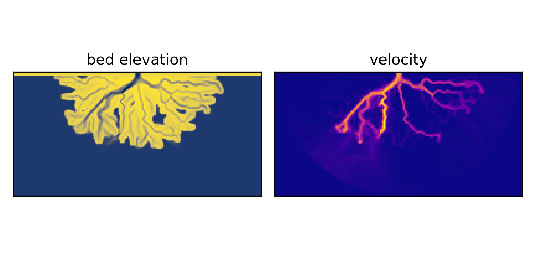
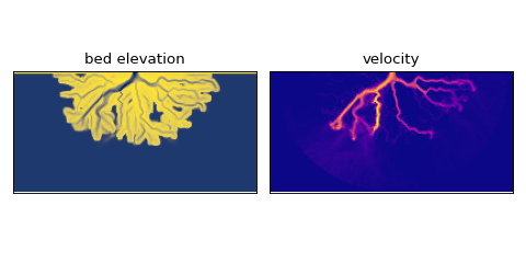
This data object is a Dataset object that can be sliced the same was as a numpy array. For example, we can slice the final bed elevation and velocity of a model run:

final_bed_elevation = data['eta'][-1, :, :]
final_velocity = data['velocity'][-1, :, :]

These slices look like this, if we were to plot them.

(png, hires.png)

Supporting documentation and files

Model reference:

• Default Model Variable Values

• Available Model Hooks

Examples:

• Simple simulation in Jupyter Notebook

• Slightly sloping basin

• Constraining subsidence to part of the domain

• Saving custom fields to the output file

References

[1]

A reduced-complexity model for river delta formation – Part 1: Modeling deltas with channel dynamics, M. Liang, V. R. Voller, and C. Paola, Earth Surf. Dynam., 3, 67–86, 2015. https://doi.org/10.5194/esurf-3-67-2015