Time in pyDeltaRCM
Time in the pyDeltaRCM model is simulated in units of seconds. The duration of a timestep is determined during model initialization to maintain numerical stability; the calculation is based on model domain and configuration parameters. The model is then iterated timestep by timestep, until an end-run condition is reached
Note
If you are using the high-level API, the model run end condition is that the elapsed model time is equal to or greater than the specified input time. As a result, the model run duration is unlikely to exactly match the input time specification, because the model timestep is unlikely to be a factor of the specified time.
Please keep this in mind when evaluating model results, and especially when comparing between different model runs.
Over the duration of the model, the water discharge (and thus sediment discharge) are assumed to be at bankfull. This assumption is based on the concept of geomorphic work [WM60] and the strongly nonlinear relationship between water discharge and sediment transport. To summarize the basis of this assumption, a very small proportion of sediment is in motion when discharge is at or near a low-flow “base flow” condition, relative to the amount of sediment in motion during flood conditions. So while flooding only occurs for a small fraction of total time, most of the time-integrated sediment transport occurs during this fraction of time, and the remainder of time is deemed negligible in comparison.
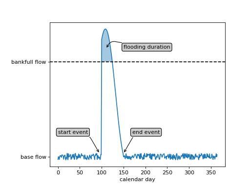
For example, in the contrived river-delta hydrograph shown below, the discharge fluctuates around a base-flow condition for most of the year, with the exception of a 50 day period when a flood event occurs (from “start event” to “end event”). For 25 days of the flood event, the discharge is high enough to exceed the bankfull discharge (“flooding duration”).

A numerical model could simulate every day of this hydrograph, but this would require substantial computing power. To accelerate the computation time of models, we assume that the only important period of time is when the river is at-or-above bankfull discharge, and we collapse the hydrograph to a single value: the bankfull discharge. The choice of bankfull discharge for the single-value discharge assumption is a matter of convenience, in that this is readily estimated from field data or measurements.
The duration of time represented by the single-value discharge assumption is also determined by the hydrograph. We arrive at the so-called intermittency factor (\(I_f\)) by finding the fraction of unit-time per unit-time when the river is in flood. For this example, the intermittency factor scales between days and years as
The intermittency factor thus gives a relationship to scale pyDeltaRCM model time (which is always computed in units of seconds elapsed) from seconds to years. For example, for a model run that has elapsed \(4.32 \times 10^8\) seconds and an assumed intermittency factor of 0.07:
Note
A convenience function is supplied with the low-level API for these time conversions: scale_model_time.
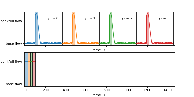
Applying the intermittency assumption to a four year model simulation reveals the computational advantage of this approach. A simulation of every day in the simulation duration would require 1460 days of simulated time (\(1.26 \times 10^8\) seconds).

In contrast, by condensing the simulated time down to a bankfull discharge only, the intermittency assumption allows us to simulate the same “four year” period in just under 59 days of simulated time (\(5.08 \times 10^6\) seconds).
See also
References
Wolman, M. G., & Miller, J. P. (1960). Magnitude and frequency of forces in geomorphic processes. The Journal of Geology, 68(1), 54–74. https://doi.org/10.1086/626637