User Guide

This documentation provides some “workflow” examples as well as some explanations and background about the various methods available in DeltaMetrics.

Setting up your coding environment

All of the documentation in this package assumes that you have imported the DeltaMetrics package as dm:

>>> import deltametrics as dm

Additionally, we frequently rely on the numpy package, and matplotlib. We will assume you have imported these packages by their common shorthand as well; if we import other packages, or other modules from matplotlib, these imports will be declared!

>>> import numpy as np
>>> import matplotlib.pyplot as plt

Create and manipulate a “DataCube”

DeltaMetrics centers around the use of “Cubes”. In DeltaMetrics, these Cube objects are the central office that connects all the different modules and a workflow together. The base cube is the DataCube, which is set up to handle multi-variable three-dimensional datasets; for example, 2D-spatial timeseries data of multiple variables.

The data of the DataCube can come from a file or can be directly passed; where possible, loading from a file is usually preferred, because it is memory-efficient. Connecting to a netCDF file on disk is as simple as:

>>> acube = dm.cube.DataCube('/path/to/data/file.nc')

Hint

For more information about data files, and how to configure your data to work with DeltaMetrics, please visit the Examples/io section of the documentation.

For this guide to be easy to follow along with, we will use some sample data that comes with DeltaMetrics.

>>> golfcube = dm.sample_data.golf()
>>> golfcube
<deltametrics.cube.DataCube object at 0x...>

Creating the golfcube connects to a dataset on your computer (the file is downloaded if it has not already been downloaded). Creating the DataCube though, does not read any of the data into memory, allowing for efficient computation on large datasets.

Inspect which variables are available in the golfcube.

>>> golfcube.variables
['eta', 'stage', 'depth', 'discharge', 'velocity', 'sedflux', 'sandfrac']

We can access the underlying variables by name. The returned object is an xarray DataArray with coordinates matching the underlying data source. Per xarray, the underlying data field contains a numpy array. For example, access variables as:

>>> type(golfcube['eta'])
<class 'xarray.core.dataarray.DataArray'>
>>> type(golfcube['eta'].data)
<class 'numpy.ndarray'>
>>> golfcube['eta'].shape
(101, 100, 200)

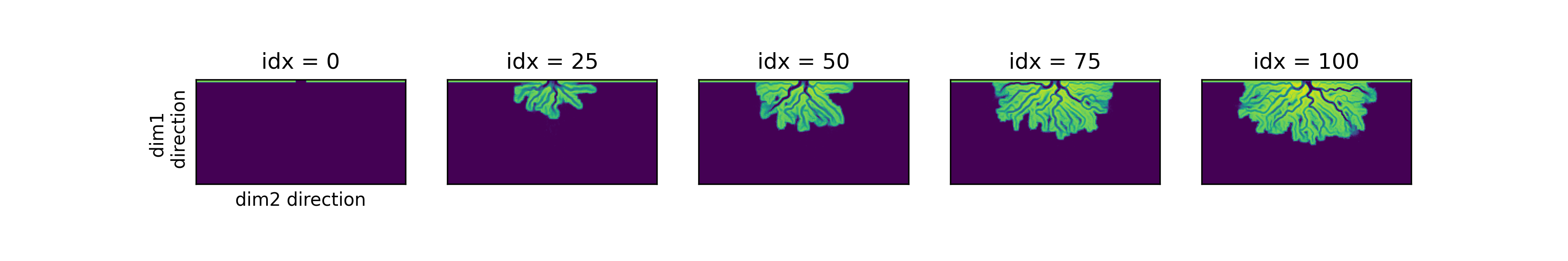
Examine a timeseries of bed elevation by taking slices out of the eta variable; we can slice the underlying data directly with an index, the same as a numpy array. Remember that time is ordered along the 0th dimension.

>>> # set up indices to slice the cube
>>> nt = 5
>>> t_idxs = np.linspace(0, golfcube.shape[0]-1, num=nt, dtype=int)  # linearly interpolate t_idxs
...
>>> # make the plot
>>> fig, ax = plt.subplots(1, nt, figsize=(12, 2))
>>> for i, idx in enumerate(t_idxs):
...     ax[i].imshow(golfcube['eta'][idx, :, :], vmin=-2, vmax=0.5)  # show the slice
...     ax[i].set_title('idx = {0}'.format(idx))
...     ax[i].set_xticks([])
...     ax[i].set_yticks([])
>>> ax[0].set_ylabel('dim1 \n direction')
>>> ax[0].set_xlabel('dim2 direction')
>>> plt.show()

(png, hires.png)

Note

The 0th dimension of the cube must be the time dimension, and the 1st and 2nd dimensions represent the spatial dimensions of the data domain, but can have any arbitrary “name” for the dimensions. For example, from pyDeltaRCM the 1st and 2nd dimensions are named x and y respectively (x is considered a downstream coordinate in that model). In DeltaMetrics, we refer to these spatial dimensions as dim1 and dim2, because they may have any name.

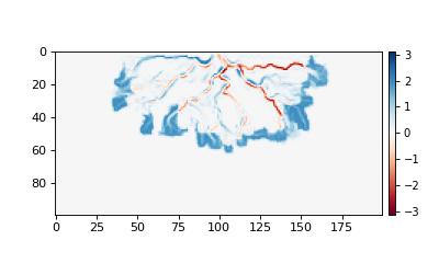
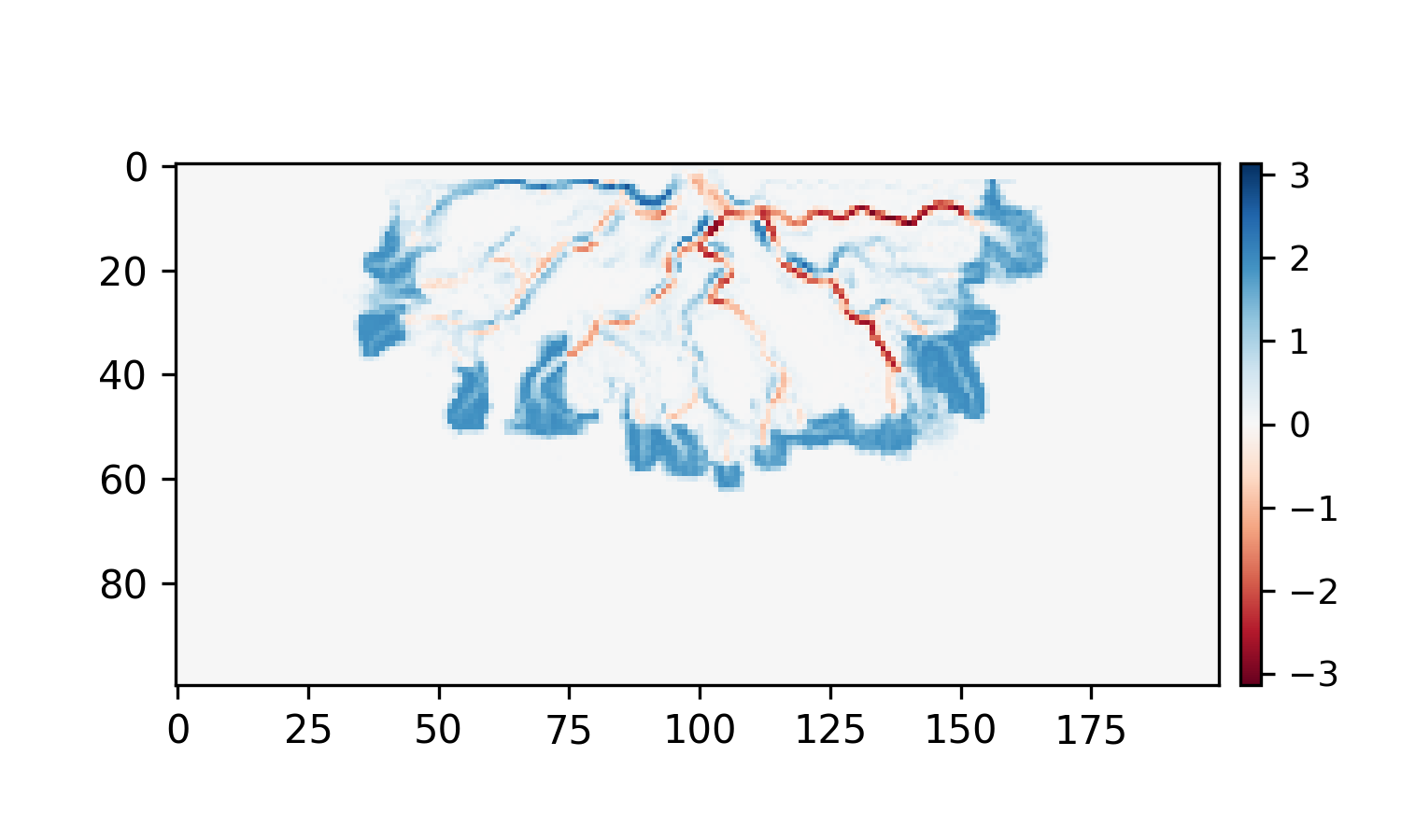
The CubeVariable supports arbitrary math (using xarray). For example:

>>> # compute the change in bed elevation between the last two intervals above
>>> diff_time = golfcube['eta'][t_idxs[-1], :, :] - golfcube['eta'][t_idxs[-2], :, :]
>>> max_delta = abs(diff_time).max()
...
>>> # make the plot
>>> fig, ax = plt.subplots(figsize=(5, 3))
>>> im = ax.imshow(
...     diff_time, cmap='RdBu',
...     vmax=max_delta,
...     vmin=-max_delta)
>>> cb = dm.plot.append_colorbar(im, ax)  # a convenience function
>>> plt.show()

(png, hires.png)

Manipulating Planform data

In addition to indexing directly, slices along the Cube time dimension can be explicitly created as Planform objects. This is helpful for organizing an analysis where you want to repeatedly access data from a particular point in time.

Planform slices

Create a Planform of the last time index from the cube. The data returned from the planform are an xarray DataArray, so you can continue to perform arbitrary math on the data.

>>> final = dm.plan.Planform(golfcube, idx=-1)
>>> final.shape
(100, 200)
>>> final['eta']
<xarray.DataArray 'eta' (x: 100, y: 200)>
array([[ 0.015 ,  0.015 ,  0.015 , ...,  0.015 ,  0.015 ,  0.015 ],
       [ 0.0075,  0.0075,  0.0075, ...,  0.0075,  0.0075,  0.0075],
       [ 0.    ,  0.    ,  0.    , ...,  0.    ,  0.    ,  0.    ],
       ...,
       [-2.    , -2.    , -2.    , ..., -2.    , -2.    , -2.    ],
       [-2.    , -2.    , -2.    , ..., -2.    , -2.    , -2.    ],
       [-2.    , -2.    , -2.    , ..., -2.    , -2.    , -2.    ]],
      dtype=float32)
Coordinates:
    time     float32 5e+07
  * x        (x) float32 0.0 50.0 100.0 150.0 ... 4.85e+03 4.9e+03 4.95e+03
  * y        (y) float32 0.0 50.0 100.0 150.0 ... 9.85e+03 9.9e+03 9.95e+03
Attributes:
    slicetype:           data_planform
    knows_stratigraphy:  False
    knows_spacetime:     True

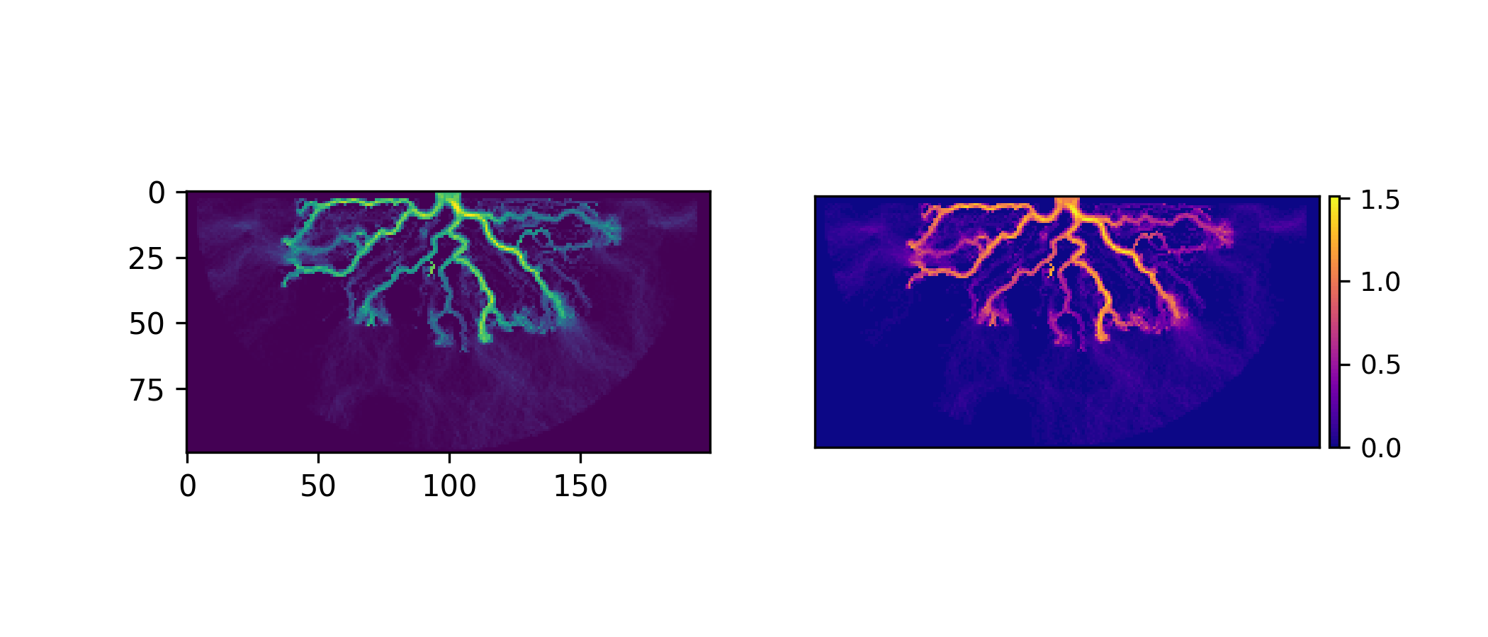
You can visualize the data yourself, or use the built-in show() method of a Planform.

>>> fig, ax = plt.subplots(1, 2, figsize=(7, 3))
>>> ax[0].imshow(final['velocity'])   # display directly
>>> final.show('velocity', ax=ax[1])  # use the built-in show()
>>> plt.show()

(png, hires.png)

Hint

Do Planform objects seems too simple? They are! The basic Planform allows us to have an API consistent with the more complicated Section data (introduced below), and have a flexible standard to extend into “specialty” planforms.

Want to just slice the data directly as golfcube['eta'][-1, :, :]? Go ahead and do what works for you!

It is often helpful to associate a Planform with a Cube, to keep track of planform data from multiple points in time, or from multiple cubes. Use the register_planform() method when instantiating the Planform, or pass the object as an argument later.

>>> golfcube.register_planform('fifty', dm.plan.Planform(idx=50))

Any registered Planform can then be accessed via the planforms attribute of the Cube (returns a dict).

>>> golfcube.planforms['fifty']
<deltametrics.plan.Planform object at 0x...>

Specialty Planform objects

A slice of the Cube is a basic Planform, but often there are some analyses we wish to compute on a Planform, that may have multiple steps and sets of derived values we want to keep track of. DeltaMetrics has several specialty planform objects that make this easier. These specialty calculations are beyond the scope of this basic user guide, find more information on the Planform API reference page.

Manipulating Section data

Similar to Planform slices, we can make cuts across the Cube time dimension with Section objects. Most often, it’s best to use the API to register a section of a specified type to an underlying data cube and assigning it a name (“demo” below). Registered sections are accessed via the sections attribute of the cube:

For a data cube, sections are most easily instantiated by the register_section method:

>>> golfcube.register_section('demo', dm.section.StrikeSection(distance_idx=10))

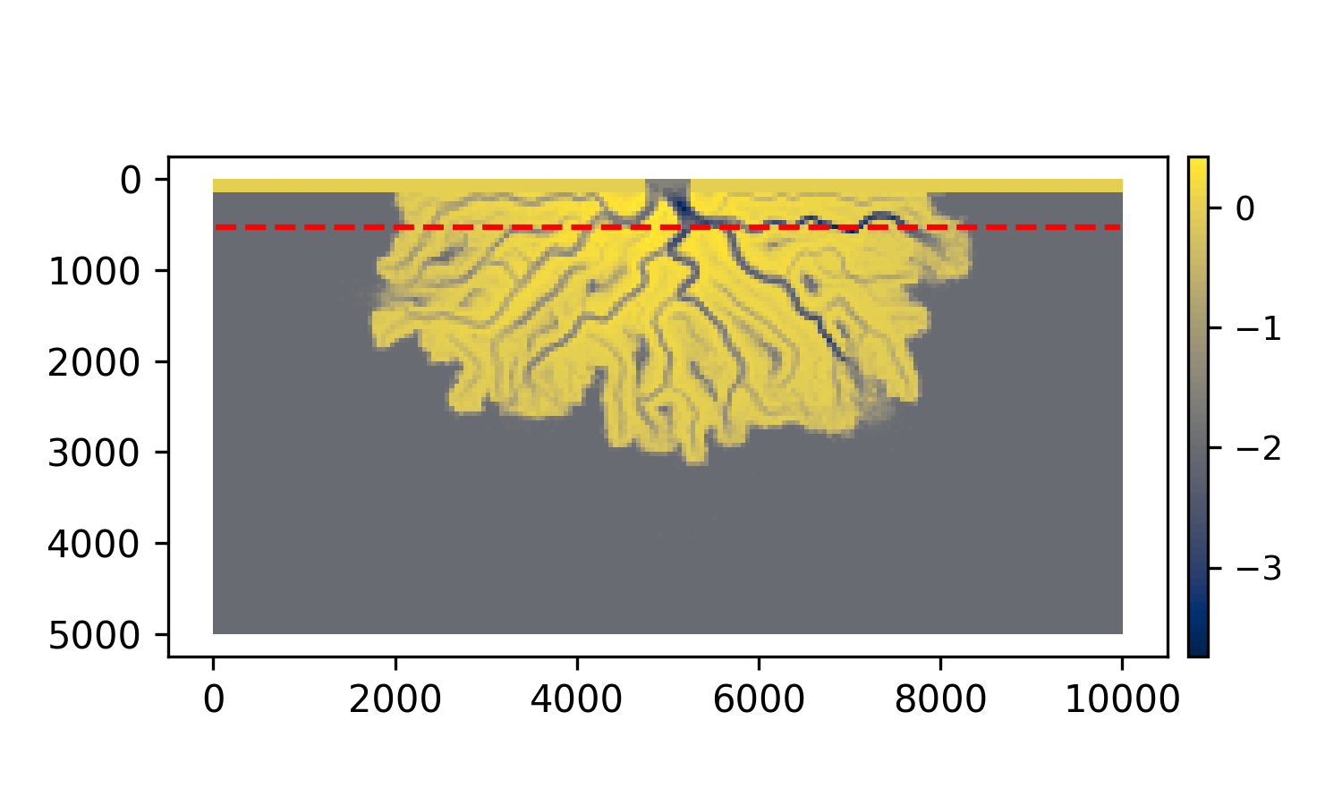
which creates a section across a constant y-value ==10. The path of any Section in the x-y plane can always be accessed via the .trace attribute. We can plot the trace on top the the final bed elevation to see where the section will be located.

>>> fig, ax = plt.subplots()
>>> golfcube.quick_show('eta', idx=-1, ax=ax, ticks=True)
>>> ax.plot(golfcube.sections['demo'].trace[:,0],
...         golfcube.sections['demo'].trace[:,1], 'r--') 
>>> plt.show() 

(png, hires.png)

Any registered section can then be accessed via the sections attribute of the Cube (returns a dict).

>>> golfcube.sections['demo']
<deltametrics.section.StrikeSection object at 0x...>

Available section types are PathSection, StrikeSection, DipSection, and RadialSection. Notably, Sections do not refer to any variable in particular, so Sections are sliced themselves, similarly to the cube.

>>> golfcube.register_section('demo', dm.section.StrikeSection(distance_idx=10))
>>> golfcube.sections['demo']['velocity']
<xarray.DataArray 'velocity' (time: 101, s: 200)>
array([[0.2   , 0.2   , 0.2   , ..., 0.2   , 0.2   , 0.2   ],
       [0.    , 0.    , 0.    , ..., 0.    , 0.    , 0.    ],
       [0.    , 0.0025, 0.    , ..., 0.    , 0.    , 0.    ],
       ...,
       [0.    , 0.    , 0.    , ..., 0.0025, 0.    , 0.    ],
       [0.    , 0.    , 0.    , ..., 0.    , 0.    , 0.    ],
       [0.    , 0.    , 0.    , ..., 0.0025, 0.    , 0.    ]],
      dtype=float32)
Coordinates:
  * s        (s) float64 0.0 50.0 100.0 150.0 ... 9.85e+03 9.9e+03 9.95e+03
  * time     (time) float32 0.0 5e+05 1e+06 1.5e+06 ... 4.9e+07 4.95e+07 5e+07
Attributes:
    slicetype:           data_section
    knows_stratigraphy:  False
    knows_spacetime:     True

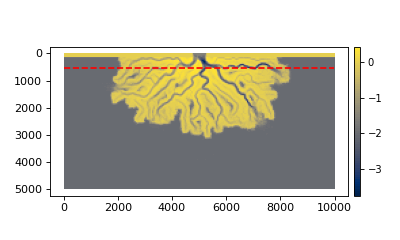
We can visualize sections:

>>> fig, ax = plt.subplots(3, 1, sharex=True, figsize=(12,6))
>>> golfcube.show_section('demo', 'eta', ax=ax[0])
>>> golfcube.show_section('demo', 'velocity', ax=ax[1])
>>> golfcube.show_section('demo', 'sandfrac', ax=ax[2])
>>> plt.show() 

(png, hires.png)

You can also create a standalone section, which is not registered to the cube, but still supports slicing from the underlying dataset.

>>> sass = dm.section.StrikeSection(golfcube, distance_idx=10)
>>> np.all(sass['velocity'] == golfcube.sections['demo']['velocity']) 
True

“Quick” stratigraphy

We are often interested in not only the spatiotemporal changes in the planform of the delta, but we want to know what is preserved in the subsurface. In DeltaMetrics, we refer to this preserved history as the “stratigraphy”, and we provide a number of convenient routines for computing stratigraphy and analyzing deposits.

Importantly, stratigraphy (or i.e., which voxels are preserved) is not computed by default when a Cube instance is created. We must directly tell the Cube instance to compute stratigraphy by specifying which variable contains the bed elevation history, because this history dictates preservation. We have implemented support for rapid stratigraphy computation for visualization, and preserved-time statistics. These quick stratigraphy computations create a mesh of preserved elevations and fill this matrix with values sliced out of the underlying data.

Compute “quick stratigraphy” as:

>>> golfcube.stratigraphy_from('eta', dz=0.1)

Now, the DataCube has knowledge of stratigraphy, which we can further use to visualize preservation within the spacetime, or visualize as an actual stratigraphic slice.

>>> golfcube.sections['demo']['velocity'].strat.as_preserved()
<xarray.DataArray 'velocity' (time: 101, s: 200)>
array([[0.2, 0.2, 0.2, ..., 0.2, 0.2, 0.2],
       [nan, nan, nan, ..., nan, nan, nan],
       [nan, nan, nan, ..., nan, nan, nan],
       ...,
       [nan, nan, nan, ..., nan, nan, nan],
       [nan, nan, nan, ..., nan, nan, nan],
       [nan, nan, nan, ..., nan, nan, nan]], dtype=float32)
Coordinates:
  * s        (s) float64 0.0 50.0 100.0 150.0 ... 9.85e+03 9.9e+03 9.95e+03
  * time     (time) float32 0.0 5e+05 1e+06 1.5e+06 ... 4.9e+07 4.95e+07 5e+07
Attributes:
    slicetype:           data_section
    knows_stratigraphy:  True
    knows_spacetime:     True

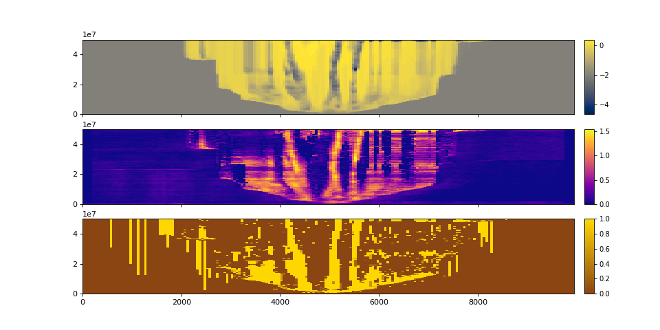
>>> fig, ax = plt.subplots(3, 1, sharex=True, figsize=(12, 8))
>>> golfcube.show_section('demo', 'velocity', ax=ax[0])
>>> golfcube.show_section('demo', 'velocity', data='preserved', ax=ax[1])
>>> golfcube.show_section('demo', 'velocity', data='stratigraphy', ax=ax[2])
>>> plt.show() 

(png, hires.png)

Quick stratigraphy makes it easy to visualize the behavior of the model across each of the variables:

>>> fig, ax = plt.subplots(5, 1, sharex=True, sharey=True, figsize=(12, 12))
>>> ax = ax.flatten()
>>> for i, var in enumerate(['time', 'eta', 'velocity', 'discharge', 'sandfrac']):
...     golfcube.show_section('demo', var, ax=ax[i], label=True,
...       style='shaded', data='stratigraphy')
>>> plt.show() 

(png, hires.png)

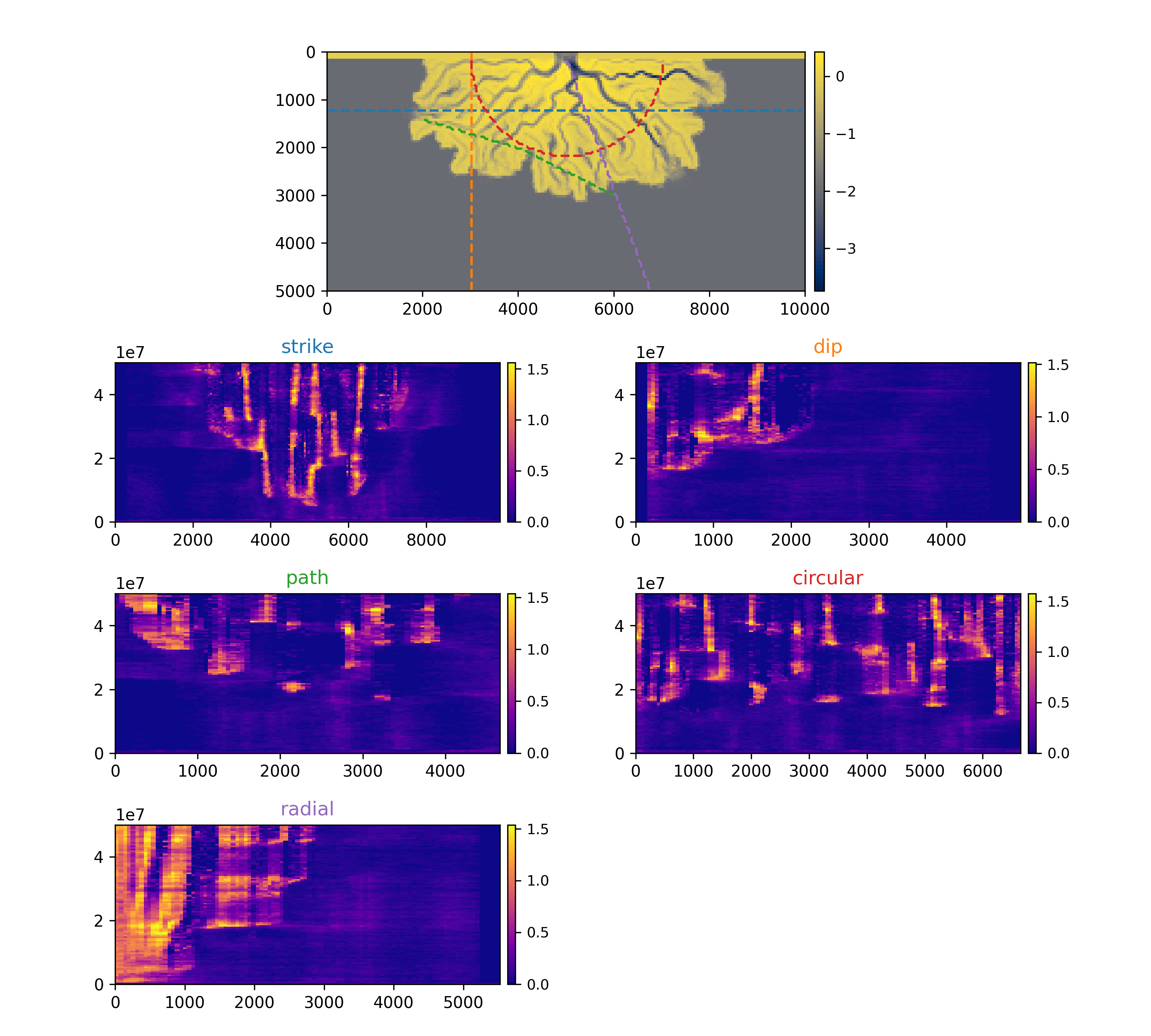
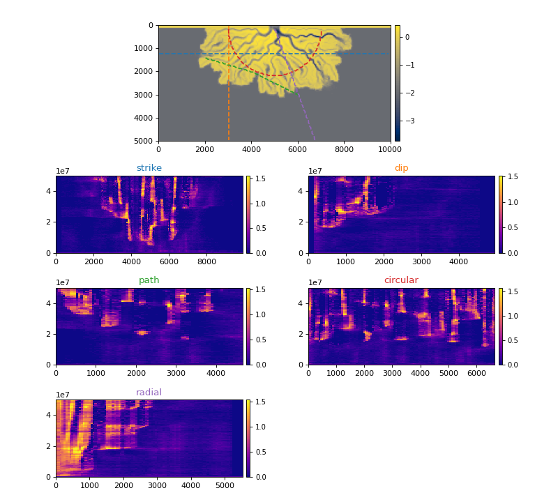
All Section types

There are multiple section types available. The Section classes all inherit from the same BaseSection class, which means they mostly have the same options available to them, and have a common API. Each Section requires unique instantiation arguments, though, which must be properly specified. The below figure shows each section type available and the velocity spacetime data extracted along that section.

>>> _strike = dm.section.StrikeSection(golfcube, distance=1200)
>>> _path = dm.section.PathSection(golfcube, path=np.array([[1400, 2000], [2000, 4000], [3000, 6000]]))
>>> _circ = dm.section.CircularSection(golfcube, radius=2000)
>>> _rad = dm.section.RadialSection(golfcube, azimuth=70)

(png, hires.png)

Default Colors in DeltaMetrics

You may have noticed the beautiful colors above, and be wondering: “how are the colors set?” We use a custom object (VariableSet) to define common plotting properties for all plots. The VariableSet supports all kinds of other controls, such as custom colormaps for any variable, addition of new defined variables, fixed color limits, color normalizations, and more. You can also use these attributes of the VariableSet in your own plotting routines.

See the default colors in DeltaMetrics here for more information.

Additionally, there are a number of plotting routines that are helpful in visualizations.

Computing and Manipulating Stratigraphy

Quick stratigraphy works great for statistics of what-is-preserved and for quick visualizations, but it has several limitations. 1) Does not consider volume of sediment filled by preserved-time indicies, 2) cannot be sliced by planform, 3) irregularity does not lend well to computation and other uses (hydrological studies).

So, we want to be able to create what I refer to as “boxy” stratigraphy. This has been done in the past by “placing” values from, e.g., sandfrac into stratigraphy. This requires full computation for any variable you want to examine though. Here, we use a method that computes boxy stratigraphy only once, then synthesizes the volume from the precomputed sparse indicies.

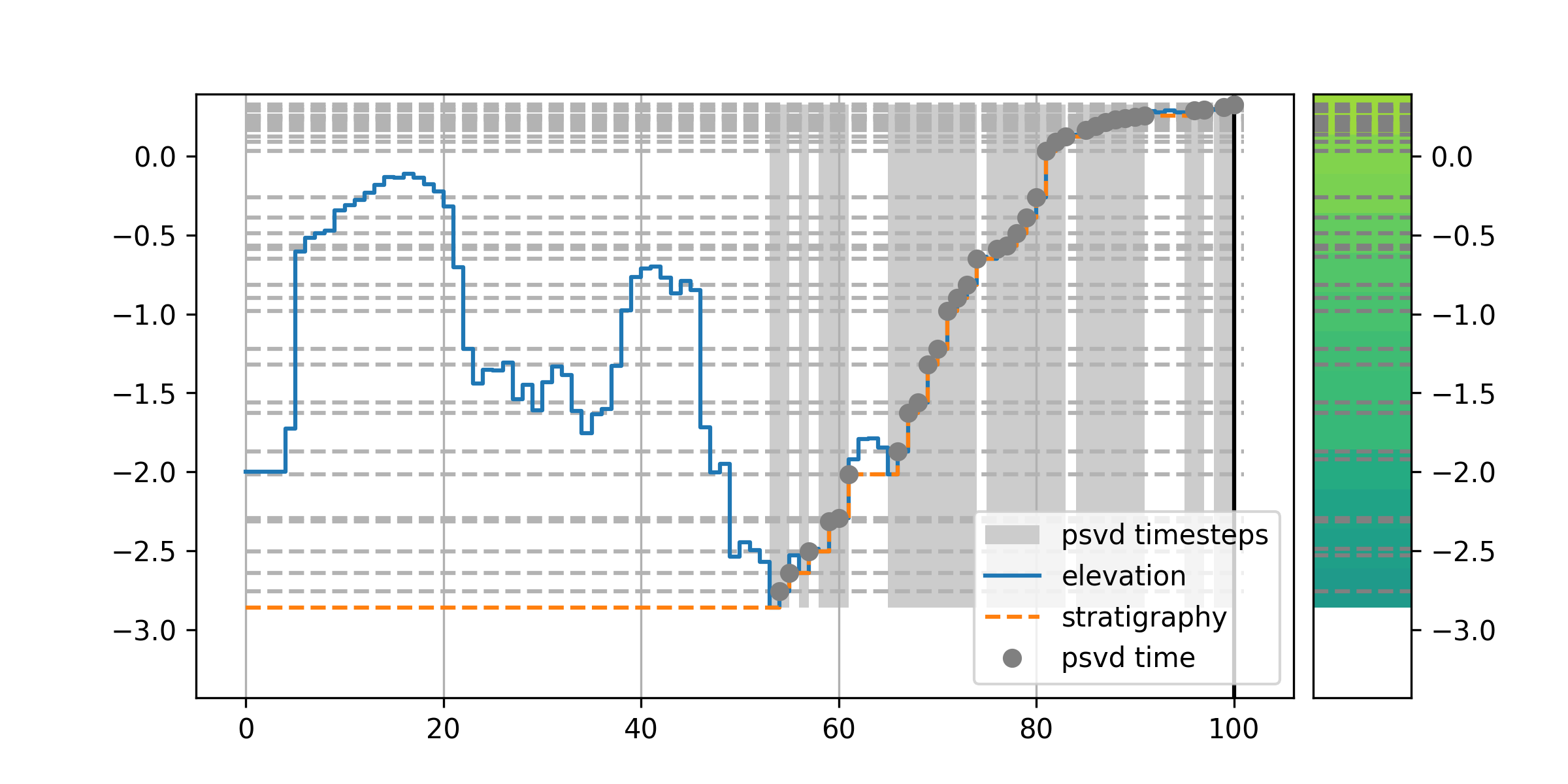
Here’s a simple example to demonstrate how we place data into the stratigraphy.

>>> ets = golfcube['eta'][:, 10, 85]  # a "real" slice of the model
>>> fig, ax = plt.subplots(figsize=(8, 4))
>>> dm.plot.show_one_dimensional_trajectory_to_strata(ets, ax=ax, dz=0.25)
>>> plt.show() 

(png, hires.png)

Begin by creating a StratigraphyCube:

>>> stratcube = dm.cube.StratigraphyCube.from_DataCube(golfcube, dz=0.05)
>>> stratcube.variables
['eta', 'stage', 'depth', 'discharge', 'velocity', 'sedflux', 'sandfrac']

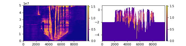
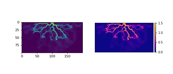
We can then slice this cube in the same way as the DataCube, but what we get back is stratigraphy rather than spacetime. Compare the slice from the golfcube (left) to the stratcube (right):

>>> fig, ax = plt.subplots(1, 2, figsize=(8, 2))
>>> golfcube.sections['demo'].show('velocity', ax=ax[0]) 
>>> stratcube.sections['demo'].show('velocity', ax=ax[1]) 
>>> plt.show() 

(png, hires.png)

Validation of the stratigraphy is easily seen by looking at the time attribute. Note that sections are not inherited from the DataCube by default (we’re working on this and related features).

Let’s add a section at the same location as golfcube.sections['demo'].

>>> stratcube.register_section('demo', dm.section.StrikeSection(distance_idx=10))
>>> stratcube.sections
{'demo': <deltametrics.section.StrikeSection object at 0x...>}

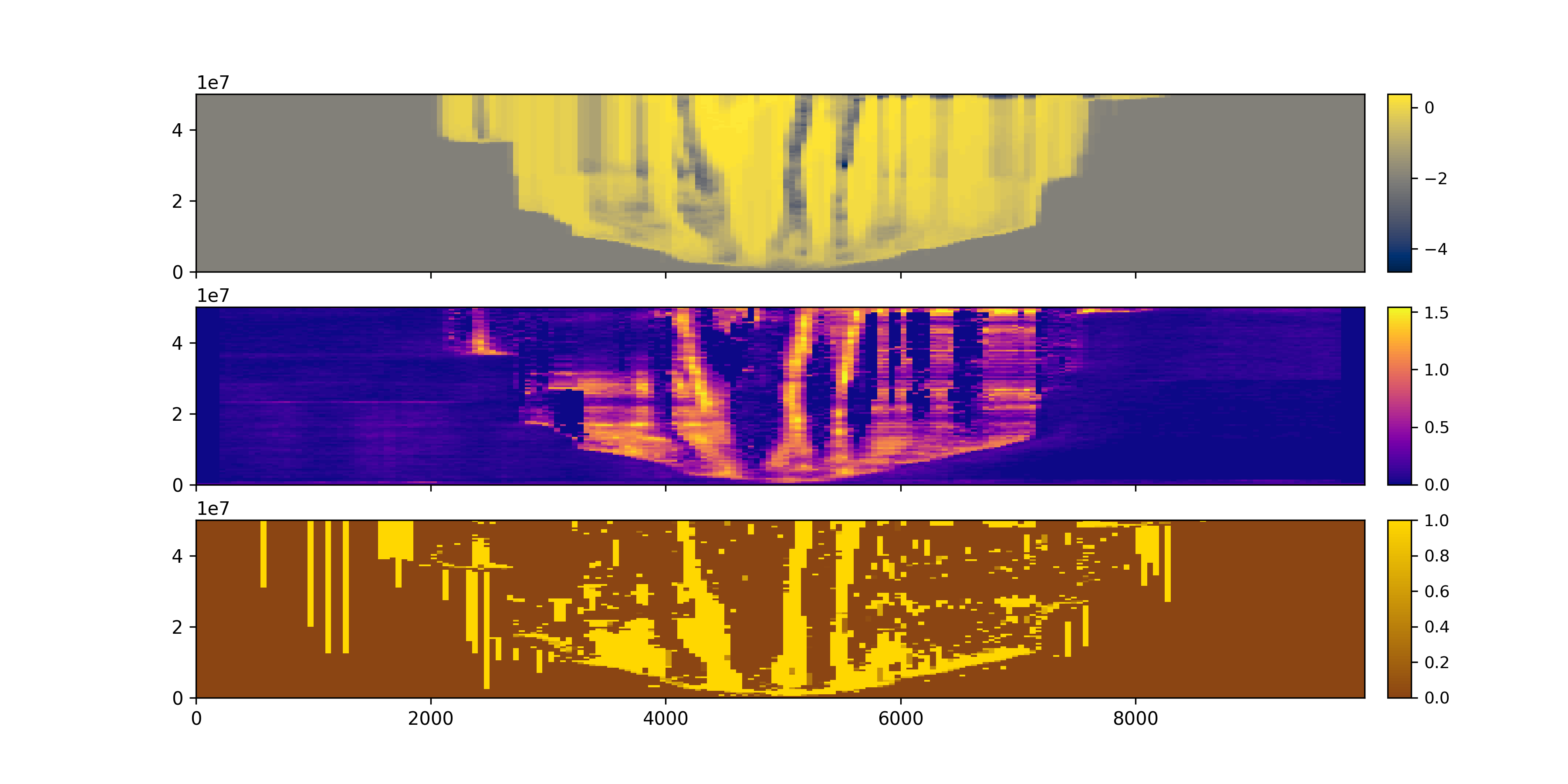
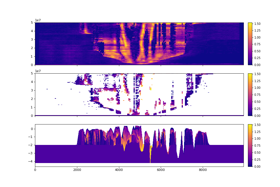
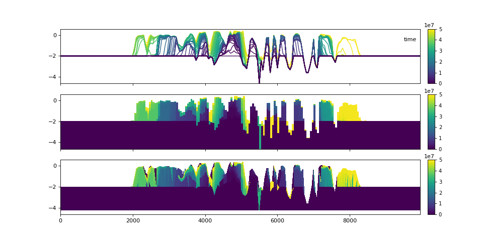
Let’s examine the stratigraphy in three different visual styles.

>>> fig, ax = plt.subplots(3, 1, sharex=True, sharey=True, figsize=(12, 8))
>>> golfcube.sections['demo'].show('time', style='lines', data='stratigraphy', ax=ax[0], label=True)
>>> stratcube.sections['demo'].show('time', ax=ax[1])
>>> golfcube.sections['demo'].show('time', data='stratigraphy', ax=ax[2])
>>> plt.show() 

(png, hires.png)

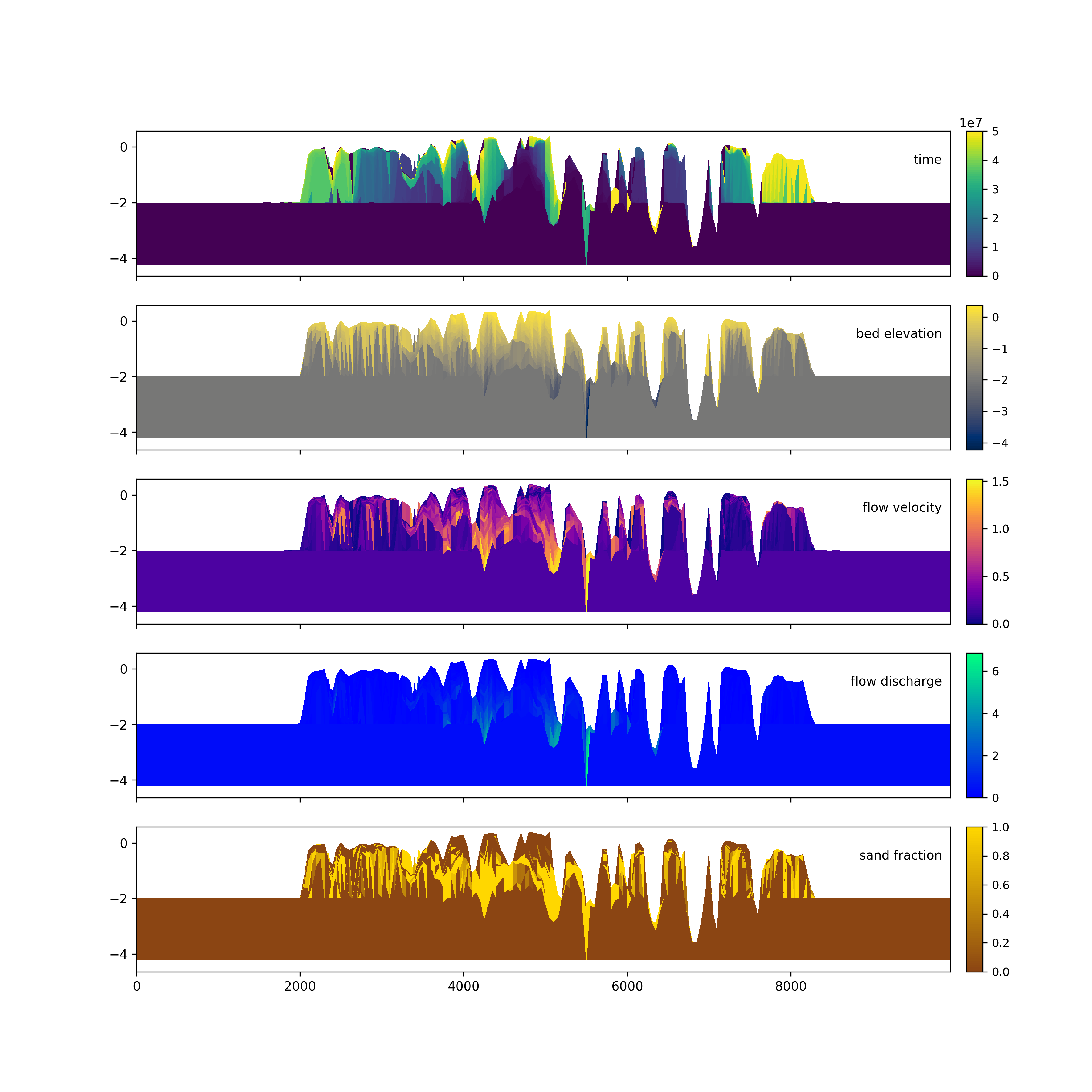
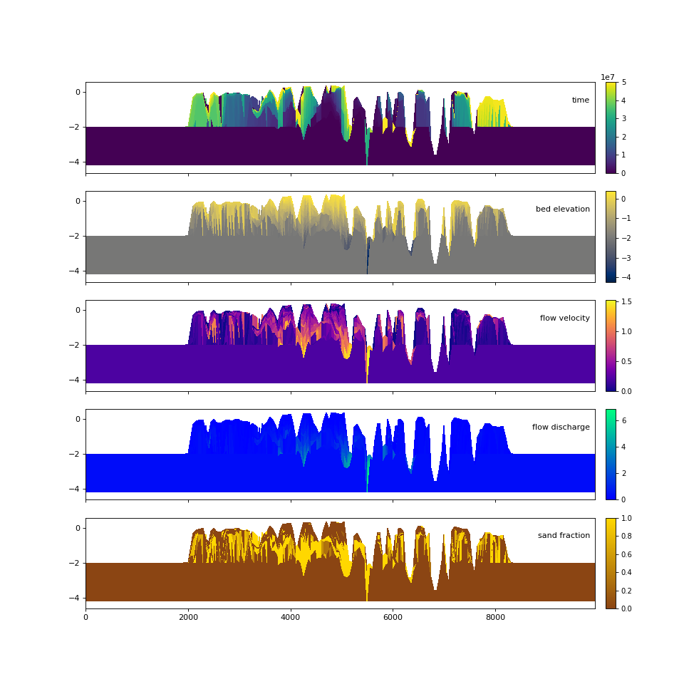
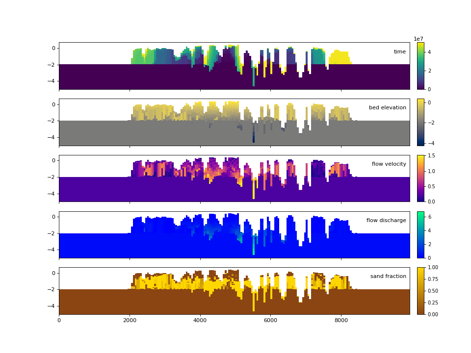
Similar to the demonstration above, each variable (property) of the underlying cube can be displayed. These displays utilize the same precomputed locations in the stratigraphy and simply filled the synthesized matrix with the different variable values.

>>> fig, ax = plt.subplots(5, 1, sharex=True, sharey=True, figsize=(12, 12))
>>> ax = ax.flatten()
>>> for i, var in enumerate(['time', 'eta', 'velocity', 'discharge', 'sandfrac']):
...     stratcube.show_section('demo', var, ax=ax[i], label=True,
...                          style='shaded', data='stratigraphy')
>>> plt.show() 

(png, hires.png)

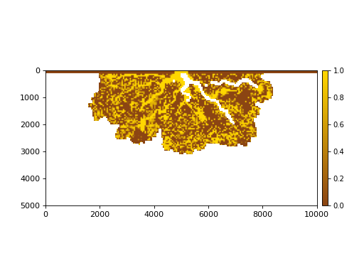
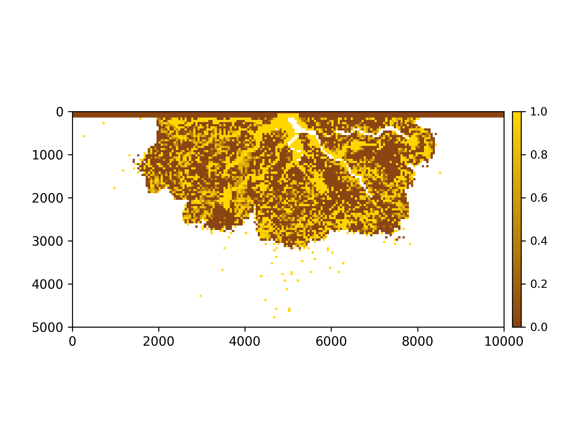
The stratigraphy cube allows us to slice Planform stratigraphy too. Specify z as the elevation of the planform slice:

>>> minus2_slice = dm.plan.Planform(stratcube, z=-2)

>>> fig, ax = plt.subplots()
>>> minus2_slice.show('sandfrac', ticks=True, ax=ax)
>>> plt.show()

(png, hires.png)

Frozen stratigraphy volumes

We still support creating “frozen” cubes, which might be useful for to speed up computations if an array is being accessed over and over.

fs = stratcube.export_frozen_variable('sandfrac')
fe = stratcube.Z  # exported volume does not have coordinate information!

fig, ax = plt.subplots(figsize=(10, 2))
pcm = ax.pcolormesh(np.tile(np.arange(fs.shape[2]), (fs.shape[0], 1)),
   fe[:,10,:], fs[:,10,:], shading='auto',
   cmap=golfcube.varset['sandfrac'].cmap,
   vmin=golfcube.varset['sandfrac'].vmin,
   vmax=golfcube.varset['sandfrac'].vmax)
dm.plot.append_colorbar(pcm, ax)
plt.show() #doctest: +SKIP

Note than you can also bypass the creation of a StratigraphyCube, and just directly obtain a frozen volume with:

>>> fs, fe = dm.strat.compute_boxy_stratigraphy_volume(golfcube['eta'], golfcube['sandfrac'], dz=0.05)

However, this will require recomputing the stratigraphy preservation to create another cube in the future, and because the StratigraphyCube stores data on disk, the memory footprint is relatively small, and so we recommend just computing the StratigraphyCube and using the export_frozen_variable) method. Finally, DataCubeVariable and StratigraphyCubeVariable support a .as_frozen() method themselves.

We should verify that the frozen cubes actually match the underlying data!

>>> np.all( fs[~np.isnan(fs)] == stratcube['sandfrac'][~np.isnan(stratcube['sandfrac'])] ) 
True

The access speed of a frozen volume is much faster than a live cube. This is because the live cube does not store any data in memory. Keeping data on disk is advantageous for large datasets, but slows down access considerably for computation. The speed of access in a frozen cube may be several thousand times faster, so it can be advantageous to export frozen cubes before computation. See a demonstration of the speed comparison in the Examples library.

Masks

We have implemented operations to compute masks of several types.

By design, masks can be instantiated directly from the most basic “raw data” components (e.g., a channel CenterlineMask from eta and velocity). This is convenient, and can be a great way to quickly explore data and prototype algorithms; however, it is often more computationally efficient to reuse a precomputed mask (and Planform objects) to compute a new mask. We describe the relationships between various Mask types, and best practices for creating each on the reference page for masks.

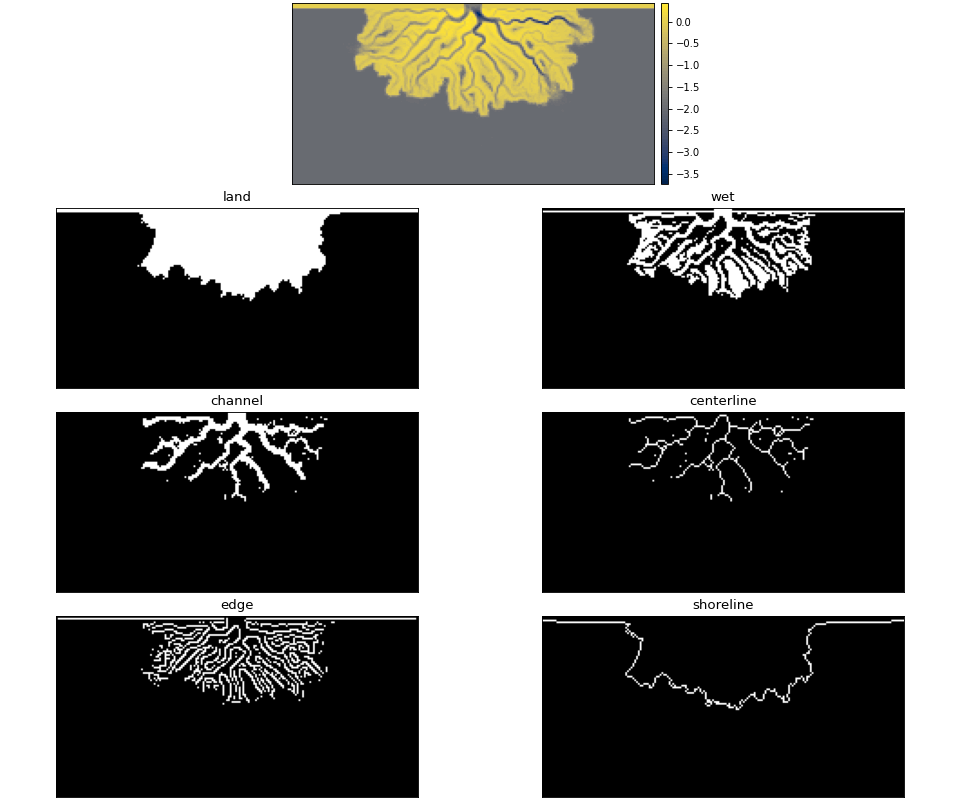
Currently implemented Masks:

• ElevationMask

• FlowMask

• LandMask

• ShorelineMask

• WetMask

• EdgeMask

• ChannelMask

• CenterlineMask

Below, we demonstrate how some of the masks can be instantiated from the most basic data components. Instantiating most masks requires a keyword parameter elevation_threshold; the exact context of this parameter may depend on the mask type, but it is often the sea-level elevation. See the reference page for each mask type if you are unsure.

# use a new cube
maskcube = dm.sample_data.golf()

# create the masks from variables in the cube
land_mask = dm.mask.LandMask(
    maskcube['eta'][-1, :, :],
    elevation_threshold=0)

wet_mask = dm.mask.WetMask(
    maskcube['eta'][-1, :, :],
    elevation_threshold=0)

channel_mask = dm.mask.ChannelMask(
    maskcube['eta'][-1, :, :],
    maskcube['velocity'][-1, :, :],
    elevation_threshold=0,
    flow_threshold=0.3)

centerline_mask = dm.mask.CenterlineMask(
    maskcube['eta'][-1, :, :],
    maskcube['velocity'][-1, :, :],
    elevation_threshold=0,
    flow_threshold=0.3)

edge_mask = dm.mask.EdgeMask(
    maskcube['eta'][-1, :, :],
    elevation_threshold=0)

shore_mask = dm.mask.ShorelineMask(
    maskcube['eta'][-1, :, :],
    elevation_threshold=0)

(png, hires.png)