Getting started with a 10-minute tutorial

This documentation provides a guide to learn the most basic components of DeltaMetrics in just ten minutes! For a more in depth guide, be sure to check out the User Guide.

All of the documentation in this package assumes that you have imported the DeltaMetrics package as dm:

>>> import deltametrics as dm

Additionally, we frequently rely on the numpy package, and matplotlib. We will assume you have imported these packages by their common shorthand as well; if we import other packages, or other modules from matplotlib, these imports will be declared!

>>> import numpy as np
>>> import matplotlib.pyplot as plt

Connect to data

In your application, you will want to connect to a your own dataset, but more on that later. For now, let’s use a sample dataset that is distributed with DeltaMetrics.

>>> golfcube = dm.sample_data.golf()
>>> type(golfcube)
<class 'deltametrics.cube.DataCube'>

This creates an instance of a DataCube object, which is the simplest and most commonly used type of cube. “Cubes” in DeltaMetrics language are the central office that connects all the different modules and workflows together. Creating the golfcube connects to a dataset, but does not read any of the data into memory, allowing for efficient computation on large datasets.

Inspect which variables are available in the golfcube.

>>> golfcube.variables
['eta', 'stage', 'depth', 'discharge', 'velocity', 'sedflux', 'sandfrac']

Accessing data from a DataCube

A DataCube can be sliced directly by variable name. Slicing a cube returns an instance of CubeVariable, which is an xarray “accessor”; this means that it contains an xarray object in addition to custom functions.

>>> type(golfcube['velocity'])
<class 'xarray.core.dataarray.DataArray'>

>>> type(golfcube['velocity'].data)
<class 'numpy.ndarray'>

The underlying xarray object can be directly accessed by using a .data attribute, however, this is not necessary, and you can slice the CubeVariable directly with any valid numpy slicing style. For example, we could determine how much the average bed elevation changed at a specific location in the model domain (43, 123), by slicing the eta variable, and differencing timesteps.

>>> np.mean( golfcube['eta'][1:,43,123] - golfcube['eta'][:-1,43,123] )
<xarray.DataArray 'eta' ()> Size: 4B
array(0., dtype=float32)
Coordinates:
    x        float32 4B 2.15e+03
    y        float32 4B 6.15e+03

The DataCube is often used by taking horizontal or vertical “cuts” of the cube. In this package, we refer to horizontal cuts as “plans” (Planform data) and vertical cuts as “sections” (Section data).

The Planform and Section data types have a series of helpful classes and functions, which are fully documented in their respective pages.

Planform data

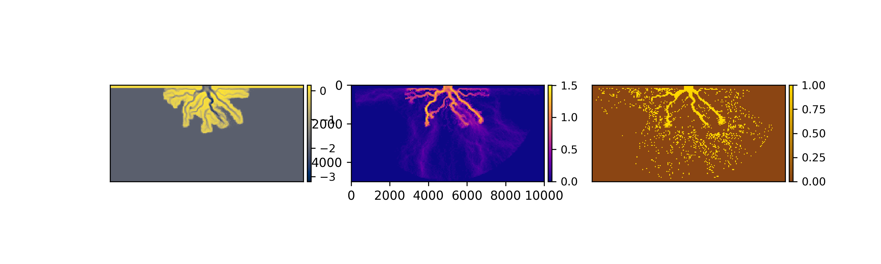
We can visualize Planform data of the cube with a number of built-in functions. Let’s inspect the state of several variables of the Cube at the fortieth (40th) timestep:

Note

This API will change to be consistent with the show_section API below. Users will register_plan and then call it, or pass a freshly instantiated plan instance.

>>> import matplotlib.pyplot as plt

>>> fig, ax = plt.subplots(1, 3)
>>> golfcube.quick_show('eta', idx=40, ax=ax[0])
>>> golfcube.quick_show('velocity', idx=40, ax=ax[1], ticks=True)
>>> golfcube.quick_show('sandfrac', idx=40, ax=ax[2])
>>> plt.show() 

(png, hires.png)

Section data

We are often interested in not only the spatiotemporal changes in the planform of the delta, but we want to know what is preserved in the subsurface. In DeltaMetrics, we refer to this preserved history as the “stratigraphy”, and we provide a number of convenient routines for computing stratigraphy and analyzing the deposits.

Importantly, the stratigraphy (or i.e., which voxels are preserved) is not computed by default when a Cube instance is created. We must directly tell the Cube instance to compute stratigraphy by specifying which variable contains the bed elevation history, because this history dictates preservation.

>>> golfcube.stratigraphy_from('eta', dz=0.1)

For this example, the stratigraphic computation is relatively fast (< one second), but for large data domains covering a large amount of time, this computation may not be as fast. The stratigraphy computed via stratigraphy_from is often referred to as “quick” stratigraphy, and may be helpful for visualizing cross sections of the deposit, but we recommend creating a StratigraphyCube from a DataCube for thorough analysis of stratigraphy.

For the sake of simplicity, this documentation uses the StrikeSection as an example Section type, but the following lexicon generalizes across all of the Section classes.

For a data cube, sections are most easily instantiated by the register_section method:

>>> golfcube.register_section('demo', dm.section.StrikeSection(distance_idx=10))

which can then be accessed via the sections attribute of the Cube.

>>> golfcube.sections['demo']
<deltametrics.section.StrikeSection object at 0x...>

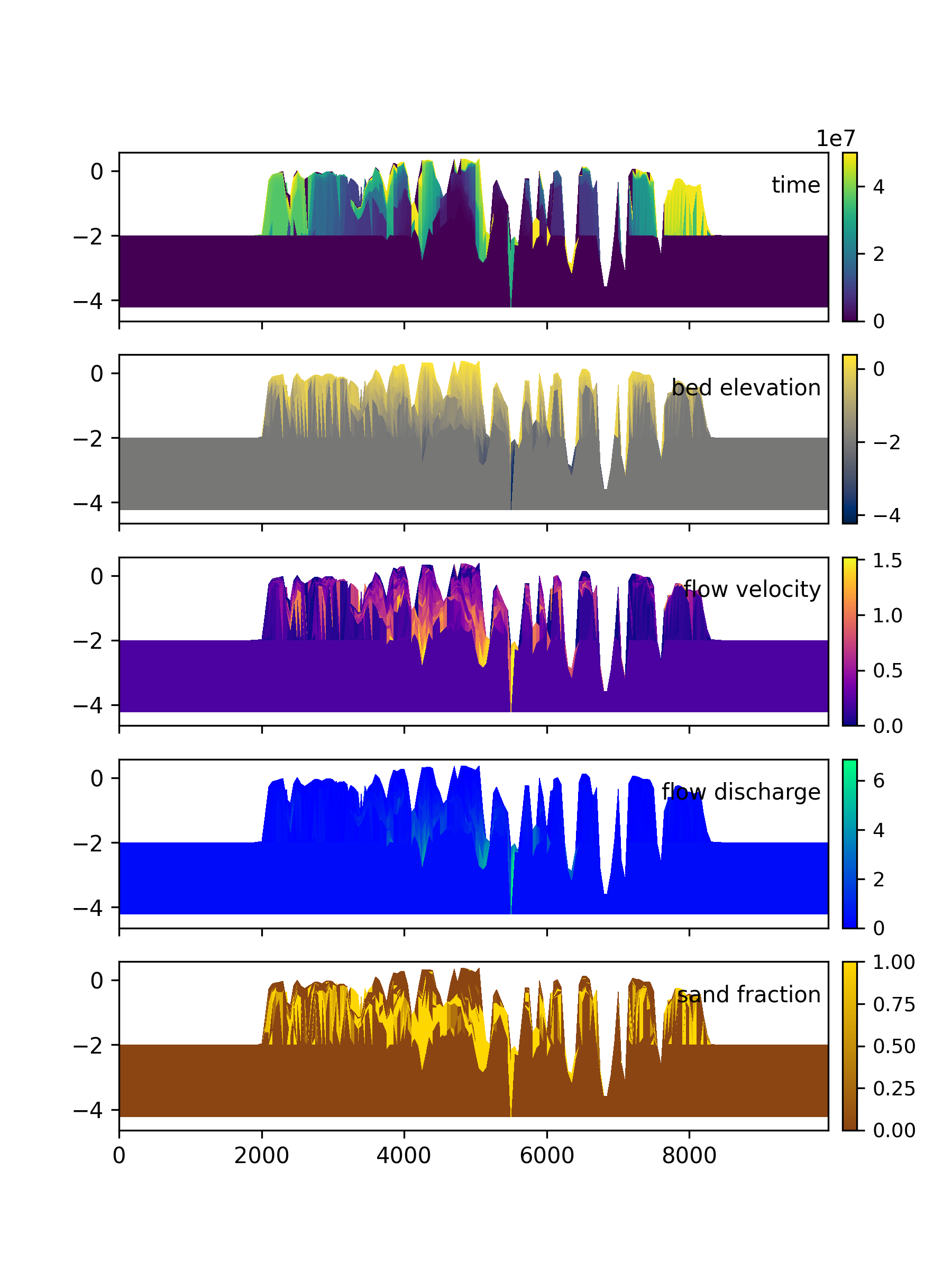
Using the “quick” stratigraphy, we can visualize a few of the available data variables as stratigraphy:

>>> fig, ax = plt.subplots(5, 1, sharex=True, figsize=(8,5))
>>> ax = ax.flatten()
>>> for i, var in enumerate(['time', 'eta', 'velocity', 'discharge', 'sandfrac']):
...    golfcube.show_section('demo', var, data='stratigraphy', ax=ax[i], label=True)
>>> plt.show() 

(png, hires.png)