Plotting operations

The package uses a few utility classes and functions to make consistent plotting easy thoughout the package. This reference page documents the lower-level utilities used to make this happen.

Note

The built-in routines to plot Section and Plan objects are not documented here, look for documentation on those high-level methods in their respective module documentation.

Hint

There is a complete Visualization Guide about the organization of this area of DeltaMetrics and examples for how to use and make visualizations.

The functions are defined in deltametrics.plot.

Default styling

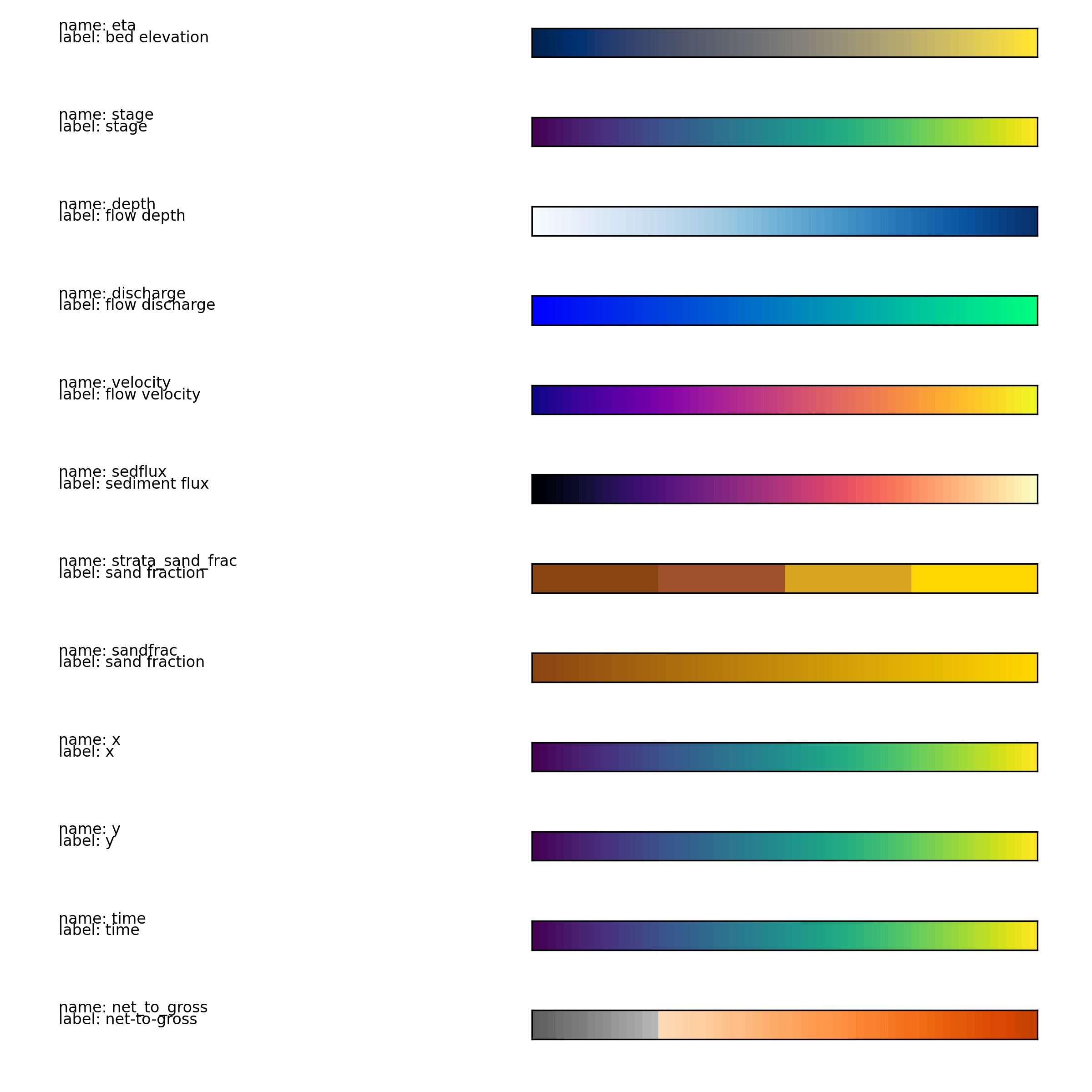
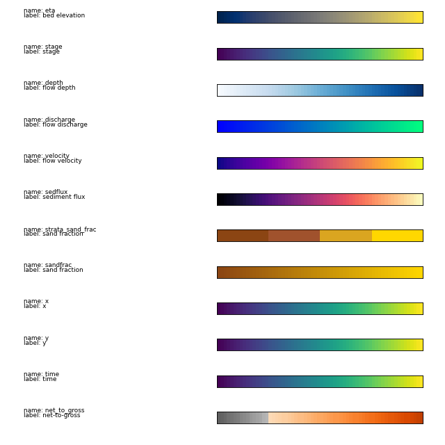
By default, each variable receives a set of styling definitions. The default parameters of each styling variable are defined below:

(png, hires.png)

Plotting utility objects

These objects are mostly used internally to help make plots appear consistent across the library. You may want to examine these to change the style of plotting across the package.

VariableInfo(name, **kwargs)	Variable styling and information.
VariableSet([override_dict])	A default set of properties for variables.

Plotting convenience functions

These functions may be helpful in making figures and exploring during analyses. Mostly, these functions provide a component of a plot.

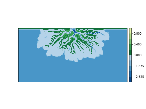
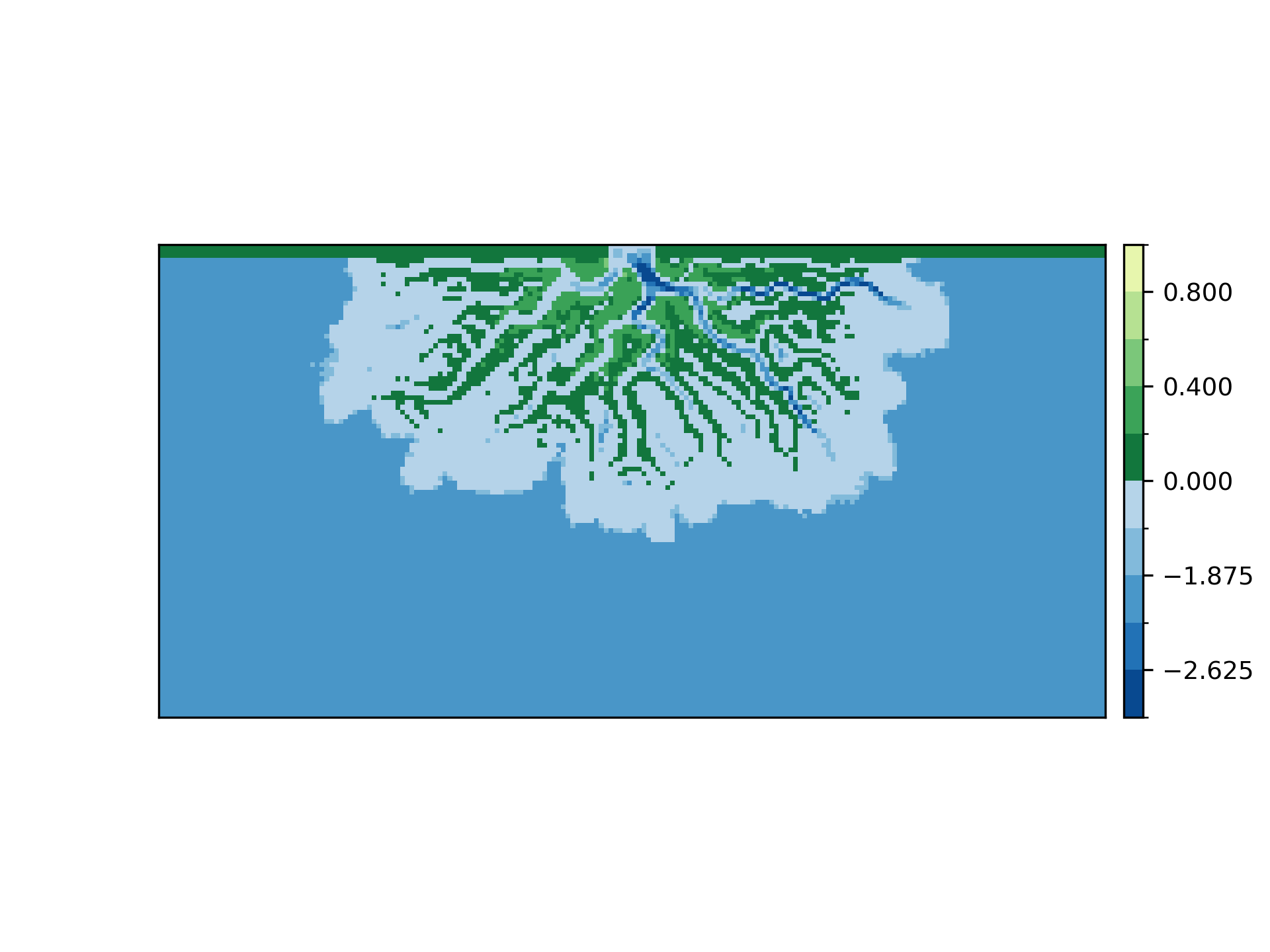
deltametrics.plot.aerial_view(elevation_data, datum=0, ax=None, ticks=False, colorbar_kw={}, return_im=False, **kwargs)

Show an aerial plot of an elevation dataset.

See also: implementation wrapper for a cube.

Parameters:

• elevation_data – 2D array of elevations.

• datum – Sea level reference, default value is 0.

• ax (Axes object, optional) – A matplotlib Axes object to plot the section. Optional; if not provided, a call is made to plt.gca() to get the current (or create a new) Axes object.

• ticks – Whether to show ticks. Default is false, no tick labels.

• colorbar_kw – Dictionary of keyword args passed to append_colorbar().

• return_im (bool, optional) – Returns the plt.imshow() image object if True. Default is False.

• **kwargs – Optionally, arguments accepted by cartographic_colormap(), or imshow.

Returns:

• colorbar – Colorbar instance appended to the axes.

• im (AxesImage object, optional) – Optional return of the image object itself if return_im is True

Examples

golfcube = dm.sample_data.golf()
elevation_data = golfcube['eta'][-1, :, :]

fig, ax = plt.subplots()
dm.plot.aerial_view(elevation_data, ax=ax)
plt.show()

(png, hires.png)

deltametrics.plot.overlay_sparse_array(sparse_array, ax=None, cmap='Reds', alpha_clip=(None, 90), clip_type='percentile', **kwargs)

Convenient plotting method to overlay a sparse 2D array on an image.

Should only be used with data arrays that are sparse: i.e., where many elements take the value 0 (or very near 0).

Original implementation was borrowed from the dorado project’s implementation of show_nourishment_area.

Parameters:

• sparse_array – 2d array to plot.

• ax (Axes object, optional) – A matplotlib Axes object to plot the section. Optional; if not provided, a call is made to plt.gca() to get the current (or create a new) Axes object.

• cmap – Maplotlib colormap to use. String or colormap object.

• alpha_clip – Two element tuple, specifying the percentiles of the data in sparse_array to clip for display. First element specifies the lower bound to clip, second element is the upper bound. Either or both elements can be None to indicate no clipping. Default is (None, 90).

• clip_type – String specifying how alpha_clip should be interpreted. Accepted values are ‘percentile’ (default) and ‘value’. If ‘percentile’, the data in sparse_array are clipped based on the density of the data at the specified percentiles; note values should be in range [0, 100). If ‘value’, the data in sparse_array are clipped directly based on the values in alpha_clip.

Returns:

image object returned from imshow.

Return type:

image

Examples

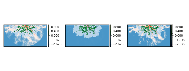
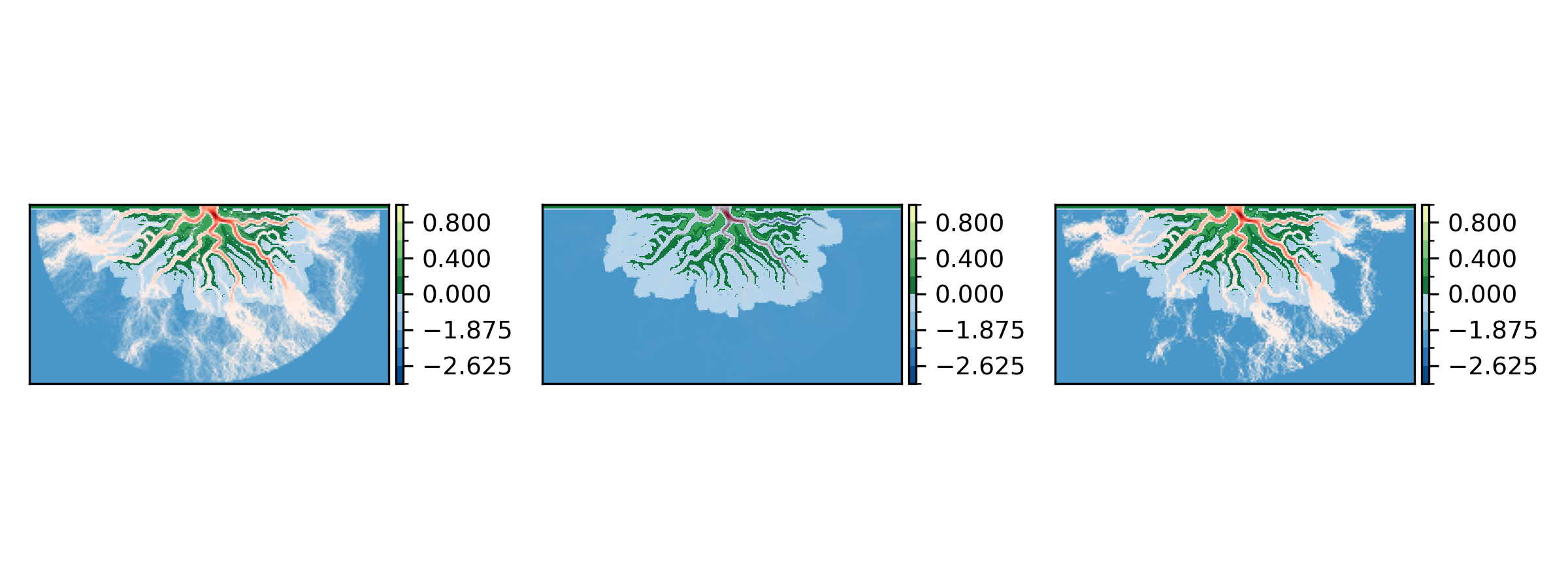
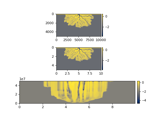
Here, we use the discharge field from the model as an example of sparse data.

golfcube = dm.sample_data.golf()
elevation_data = golfcube['eta'][-1, :, :]
sparse_data = golfcube['discharge'][-1, ...]

fig, ax = plt.subplots(1, 3, figsize=(8, 3))
for axi in ax.ravel():
    dm.plot.aerial_view(elevation_data, ax=axi)

dm.plot.overlay_sparse_array(
    sparse_data, ax=ax[0])  # default clip is (None, 90)
dm.plot.overlay_sparse_array(
    sparse_data, alpha_clip=(None, None), ax=ax[1])
dm.plot.overlay_sparse_array(
    sparse_data, alpha_clip=(70, 90), ax=ax[2])

plt.tight_layout()
plt.show()

(png, hires.png)

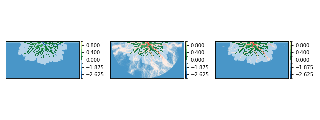
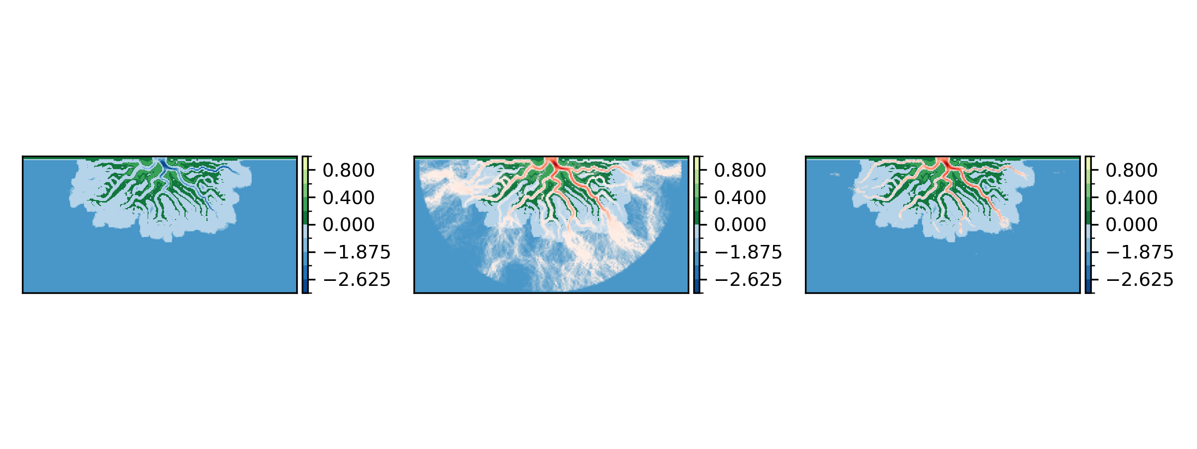
fig, ax = plt.subplots(1, 3, figsize=(8, 3))
for axi in ax.ravel():
    dm.plot.aerial_view(elevation_data, ax=axi)

dm.plot.overlay_sparse_array(
    sparse_data, ax=ax[0],
    clip_type='value')  # default clip is (None, 90)
dm.plot.overlay_sparse_array(
    sparse_data, ax=ax[1],
    alpha_clip=(None, 0.2), clip_type='value')
dm.plot.overlay_sparse_array(
    sparse_data, ax=ax[2],
    alpha_clip=(0.4, 0.6), clip_type='value')

plt.tight_layout()
plt.show()

(png, hires.png)

deltametrics.plot.style_axes_km(*args)

Style axes with kilometers, when initially set as meters.

This function can be used two ways. Passing an Axes object as the first argument and optionally a string specifying ‘x’, ‘y’, or ‘xy’ [default] will chnage the appearance of the Axes object. Alternatively, the function can be specified as the ticker function when setting a label formatter.

Parameters:

• ax (matplotlib.axes.Axes) – Axes object to format

• which (str, optional) – Which axes to style as kilometers. Default is xy, but optionally pass x or y to only style one axis.

• x (float) – If using as a function to format labels, the tick mark location.

Examples

golf = dm.sample_data.golf()

fig, ax = plt.subplots(
    3, 1,
    gridspec_kw=dict(hspace=0.5))
golf.quick_show('eta', ax=ax[0], ticks=True)

golf.quick_show('eta', ax=ax[1], ticks=True)
dm.plot.style_axes_km(ax[1])

golf.quick_show('eta', axis=1, idx=10, ax=ax[2])
ax[2].xaxis.set_major_formatter(dm.plot.style_axes_km)
# OR use: dm.plot.style_axes_km(ax[2], 'x')

plt.show()

(png, hires.png)

deltametrics.plot.append_colorbar(ci, ax, size=2, pad=2, labelsize=9, **kwargs)

Append a colorbar, consistently placed.

Adjusts some parameters of the parent axes as well.

Parameters:

• ci (matplotlib.pyplot.pcolormesh, matplotlib.pyplot.ImageAxes) – The colored object generated via matplotlib that the colormap should be stolen from.

• ax (matplotlib.Axes) – The instance of axes to place the colorbar next to.

• size (float, optional) – Width (percent of parent axis width) of the colorbar; default is 2.

• pad (float, optional) – Padding between parent and colorbar axes. Default is 0.05.

• labelsize (int, optional) – Font size of label text. Default is 9pt.

• **kwargs – Passed to matplotlib.pyplot.colorbar. For example, spacing=”proportional”.

Returns:

cb – The colorbar instance created.

Return type:

matplotlib.colorbar instance.

DeltaMetrics plot routines

These functions are similar to the convenience functions above, but mostly produce their own plots entirely, rather than adding a component of a plot.

show_one_dimensional_trajectory_to_strata(e)	1d elevation to stratigraphy.
show_histograms(*args[, sets, ax])	Show multiple histograms, including as sets.

DeltaMetrics colormaps

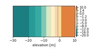
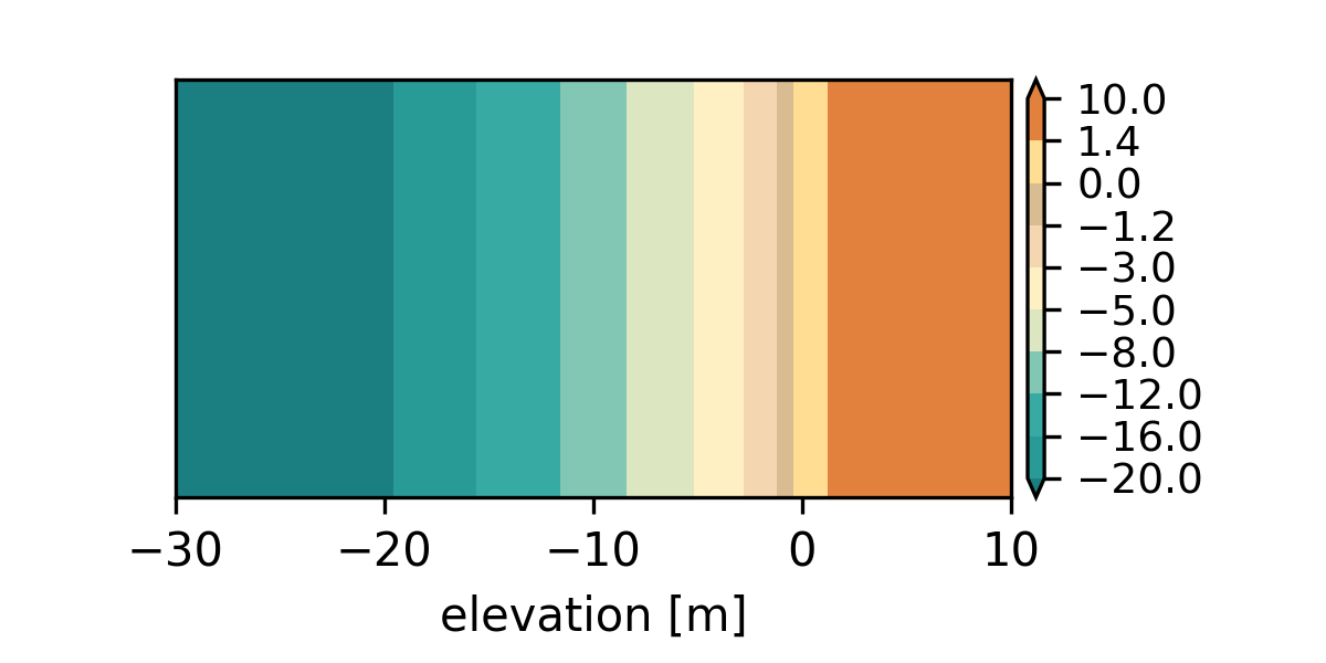
deltametrics.plot.cartographic_colormap(H_SL=0.0, h=4.5, n=1.0)

Colormap for an elevation map style.

Parameters:

• H_SL (float, optional) – Sea level for the colormap. This is the break-point between blues and greens. Default value is 0.0.

• h (float, optional) – Channel depth for the colormap. This is some characteristic below sea-level relief for the colormap to extend to through the range of blues. Default value is 4.5.

• n (float, optional) – Surface topography relief for the colormap. This is some characteristic above sea-level relief for the colormap to extend to through the range of greens. Default value is 1.0.

Returns:

• delta (matplotib.colors.ListedColormap) – The colormap object, which can then be used by other matplotlib plotting routines (see examples below).

• norm (matplotib.colors.BoundaryNorm) – The color normalization object, which can then be used by other matplotlib plotting routines (see examples below).

Examples

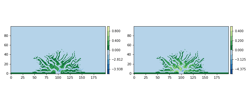
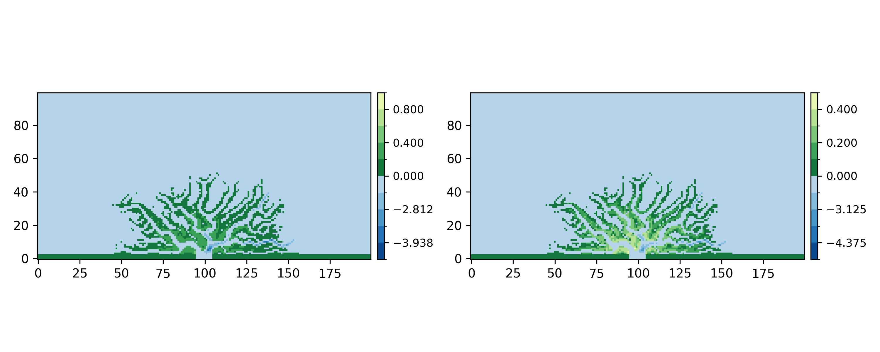
To display with default depth and relief parameters (left) and with adjust parameters to highlight depth variability (right):

golfcube = dm.sample_data.golf()

cmap0, norm0 = dm.plot.cartographic_colormap(H_SL=0)
cmap1, norm1 = dm.plot.cartographic_colormap(H_SL=0, h=5, n=0.5)

fig, ax = plt.subplots(1, 2, figsize=(10, 4))
im0 = ax[0].imshow(golfcube['eta'][-1, ...], origin='lower',
               cmap=cmap0, norm=norm0)
cb0 = dm.plot.append_colorbar(im0, ax[0])
im1 = ax[1].imshow(golfcube['eta'][-1, ...], origin='lower',
               cmap=cmap1, norm=norm1)
cb1 = dm.plot.append_colorbar(im1, ax[1])
plt.tight_layout()
plt.show()

(png, hires.png)

deltametrics.plot.aerial_colormap()

Colormap for a pesudorealistic looking aerial shot.

Warning

Not implemented.

deltametrics.plot.vintage_colormap(H_SL=0.0, h=4.5, n=1.0)

Colormap in a vintage map style.

This colormap uses a set of colors originally used by 1950s maps of the Wadden Sea [1]. The colormap is adapted from Stuart Pearson’s matlab version of the colormap [2] [3]. That colormap carries a CC BY 4.0 license.

[1]

Vinckers, J.A. Beckering. Amelander Gat (1943). Report D98 in Dutch. Rijkswaterstaat Studiedienst Hoorn, Hoorn.

[2]

Stuart Pearson. “Custom Colourmapping.” Coastally Curious (personal blog). (2022). https://coastallycurious.com/2022/02/20/custom-colourmapping/

[3]

Elias, Edwin P.L. et al. “Understanding sediment bypassing processes through analysis of high-frequency observations of Ameland Inlet, the Netherlands.” Marine Geology 415 (2019) 10.1016/j.margeo.2019.06.001

Examples

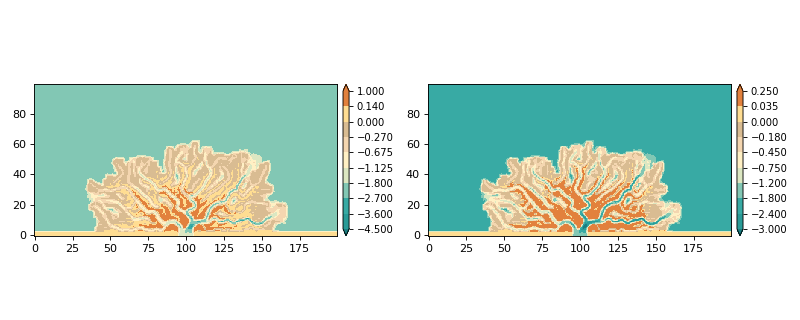
To display with default depth and relief parameters (left) and with adjust parameters to highlight depth variability (right):

golfcube = dm.sample_data.golf()

cmap0, norm0 = dm.plot.vintage_colormap(H_SL=0)
cmap1, norm1 = dm.plot.vintage_colormap(H_SL=0, h=3, n=0.25)

fig, ax = plt.subplots(1, 2, figsize=(10, 4))
im0 = ax[0].imshow(golfcube['eta'][-1, ...], origin='lower',
               cmap=cmap0, norm=norm0)
cb0 = dm.plot.append_colorbar(im0, ax[0])
im1 = ax[1].imshow(golfcube['eta'][-1, ...], origin='lower',
               cmap=cmap1, norm=norm1)
cb1 = dm.plot.append_colorbar(im1, ax[1])
plt.tight_layout()
plt.show()

(png, hires.png)

To use the colormap exactly as described in Pearson’s original publication, use parameters

cmap, norm = dm.plot.vintage_colormap(H_SL=0, h=20, n=10)

(png, hires.png)

Plotting utility functions

These functions are mostly used internally.

deltametrics.plot.get_display_arrays(VarInst, data=None)

Get arrays for display of Variables.

Function takes as argument a VariableInstance from a Section or Planform and an optional data argument, which specifies the data type to return, and gives back arrays of 1) data, 2) display x-coordinates and 3) display y-coordinates.

Parameters:

• VarInst (BaseSectionVariable subclass) – The Variable instance to visualize. May be any subclass of BaseSectionVariable or BasePlanformVariable.

• data (str, optional) – The type of data to visualize. Supported options are ‘spacetime’, ‘preserved’, and ‘stratigraphy’. Default is to display full spacetime plot for variable generated from a DataCube, and stratigraphy for a StratigraphyCube variable. Note that variables sourced from a StratigraphyCube do not support the spacetime or preserved options, and a variable from DataCube will only support stratigraphy if the Cube has computed “quick” stratigraphy.

Returns:

data, X, Y – Three matching-size ndarray representing the 1) data, 2) display x-coordinates and 3) display y-coordinates.

Return type:

ndarray

deltametrics.plot.get_display_lines(VarInst, data=None)

Get lines for display of Variables.

Function takes as argument a VariableInstance from a Section or Planform and an optional data argument, which specifies the data type to return, and gives back data and line segments for display.

Parameters:

• VarInst (BaseSectionVariable subclass) – The Variable instance to visualize. May be any subclass of BaseSectionVariable or BasePlanformVariable.

• data (str, optional) – The type of data to visualize. Supported options are ‘spacetime’, ‘preserved’, and ‘stratigraphy’. Default is to display full spacetime plot for variable generated from a DataCube. and stratigraphy for a StratigraphyCube variable. Variables from DataCube will only support stratigraphy if the Cube has computed “quick” stratigraphy.

• note:: (..) – Not currently implemented for variables from the StratigraphyCube.

Returns:

vals, segments – An off-by-one sized array of data values (vals) to color the line segments (segments). The segments are organized along the 0th dimension of the array.

Return type:

ndarray

deltametrics.plot.get_display_limits(VarInst, data=None, factor=1.5)

Get limits to resize the display of Variables.

Function takes as argument a VariableInstance from a Section or Planform and an optional data argument, which specifies how to determine the limits to return.

Parameters:

• VarInst (BaseSectionVariable subclass) – The Variable instance to visualize. May be any subclass of BaseSectionVariable or BasePlanformVariable.

• data (str, optional) – The type of data to compute limits for. Typically this will be the same value used with either get_display_arrays or get_display_lines. Supported options are ‘spacetime’, ‘preserved’, and ‘stratigraphy’.

• factor (float, optional) – Factor to extend vertical limits upward for stratigraphic sections.

Returns:

xmin, xmax, ymin, ymax – Values to use as limits on a plot. Use with, for example, ax.set_xlim((xmin, xmax)).

Return type:

float

deltametrics.plot._fill_steps(where, x=1, y=1, y0=0, **kwargs)

Fill rectangles where the boolean indicates True.

Creates an x by y matplotlib.patches.Rectangle at each index where the index i in boolean where indicates, with the lower left of the patch at (i, y0).

This utility function is utilized internally. Most often, it is used to highlight where time has been preserved (or eliminated) in a timeseries of data. For example, see show_one_dimensional_trajectory_to_strata.

Parameters:

• where (ndarray) – Boolean numpy ndarray indicating which locations to create a patch at.

• x (float) – The x-direction width of the Rectangles.

• y (float) – The y-direction height of the Rectangles.

• y0 (float) – The y-direction origin (i.e., lower-left y-value) of the Rectangles.

• **kwargs – Additional matplotlib keyword arguments passed to the Rectangle instantiation. This is where you can set most matplotlib **kwargs (e.g., color, edgecolor).

Returns:

pc – Collection of Rectangle Patch objects.

Return type:

matplotlib.patches.PatchCollection

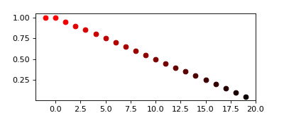
deltametrics.plot._scale_lightness(rgb, scale_l)

Utility to scale the lightness of some color.

Make a color perceptually lighter or darker. Adapted from https://stackoverflow.com/a/60562502/4038393.

Parameters:

• rgb (tuple) – A three element tuple of the RGB values for the color.

• scale_l (float) – The scale factor, relative to a value of 1. A value of 1 performs no scaling, and values less than 1 darken the color, whereas values greater than 1 brighten the color.

Returns:

scaled – Scaled color RGB tuple.

Return type:

tuple

Example

(png, hires.png)