Accounting for subsidence when computing stratigraphy

It is not uncommon for subsidence, or the sinking of the ground, to take place. When computing the preserved stratigraphy from a time-series of elevation data, a more accurate depiction of the subsurface can be developed if information about subsidence is known and accounted for. DeltaMetrics aims to provide a number of methods to incorporate subsidence data into the computed stratigraphy, allowing the user to specify a constant basin-wide rate of subsidence, or more complex spatially and temporally varying patterns. Below some examples of this functionality are shown, using synthetic 1-D elevation time-series, as well as the aeolian dune field sample dataset.

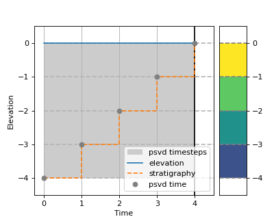
Using synthetic 1-D elevation time-series, we can create some simplified stratigraphic profiles to test our understanding of the mechanism and see whether or not the resulting stratigraphy matches our intuition. For our first example, we will consider the contrived case in which the elevation at some location is unchanging in time, however there is a constant rate of subsidence. This implies that there is indeed sedimentation occurring at this location, equivalent to the rate of subsidence. We therefore expect to see the development of a stack of stratigraphy despite there being no change in elevation, and as the processes in this example are constant in time, we expect time to be evenly preserved in the preserved stratigraphic column.

elevation = np.zeros((5,))  # elevation array of 0s

# plot 1-D trajectory w/ constant subsidence
fig, ax = plt.subplots(figsize=(5, 4))
dm.plot.show_one_dimensional_trajectory_to_strata(
    elevation, sigma_dist=1.0, ax=ax, dz=0.5)
ax.set_xlim(-0.25, 4.5)
ax.set_ylim(-4.5, 0.5)
ax.set_ylabel('Elevation')
ax.set_xlabel('Time')
plt.show()

(png, hires.png)

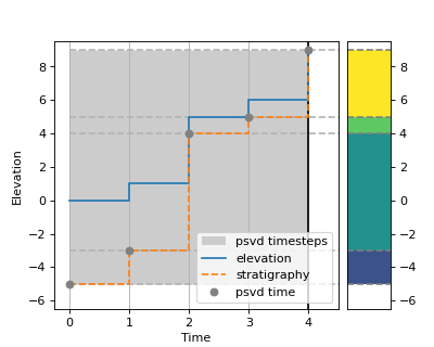
Next, using another synthetic 1-D elevation time-series, we will show how a time-varying subsidence can be accounted for when computing stratigraphy. Here we will consider a contrived case with some elevation change, and some variable subsidence. Be aware that when providing subsidence values in this manner (temporally varying values), the values provided reflect the cumulative distance subsided at that point in time.

elevation = np.array([0, 1, 5, 6, 9])

# plot 1-D trajectory w/ constant subsidence
fig, ax = plt.subplots(figsize=(5, 4))
dm.plot.show_one_dimensional_trajectory_to_strata(
    elevation, sigma_dist=np.array([1, 2, 5, 5, 6]),
    ax=ax, dz=0.5)
ax.set_xlim(-0.25, 4.5)
ax.set_ylim(-6.5, 9.5)
ax.set_ylabel('Elevation')
ax.set_xlabel('Time')
plt.show()

(png, hires.png)

Note

When a singular (integer or float) value for subsidence is provided, it is assumed that the provided value is the rate of subsidence in terms of some vertical distance per timestep. Conversely, when a time-series is provided, the each value is assumed to be the cumulative distance subsided up until that point in time. It is important to be aware of this distinction when incorporating subsidence information into the stratigraphy computation.

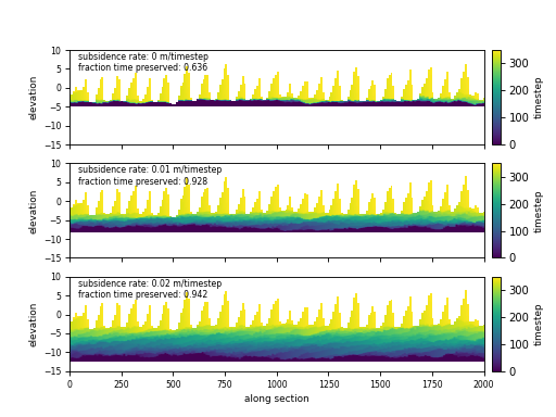
Finally, using the aeolean dataset, we will perform a similar computation to the one shown in example Aggradation and preserved time except instead of assuming some constant background aggradation rate, we will assume a constant subsidence rate. In this case, the effect steady basin-wide aggradation is equivalent to constant basin-wide subdidence.

aeolian = dm.sample_data.aeolian()

# define rates, in m/timestep
subs_rates = [0, 0.01, 0.02]

fig, ax = plt.subplots(
    len(subs_rates), 1,
    sharex=True, sharey=True)

for i, su in enumerate(subs_rates):
    # compute stratigraphy for elevation timeseries with subsidence
    vol, elev = dm.strat.compute_boxy_stratigraphy_volume(
        aeolian['eta'], aeolian['time'], sigma_dist=su,
        dz=0.1)

    # section index and calculation for preservation
    sec_idx = aeolian.shape[2] // 2
    sec_data = vol[:, :, sec_idx]
    sec_data_flat = sec_data[~np.isnan(sec_data)]
    fraction_preserved = (len(np.unique(sec_data_flat)) / aeolian.shape[0])

    # show a slice through the section
    im = ax[i].imshow(
        vol[:, :, sec_idx],
        extent=[0, aeolian.dim1_coords[-1], elev.min(), elev.max()],
        aspect='auto', origin='lower')
    cb = dm.plot.append_colorbar(im, ax=ax[i])
    cb.ax.set_ylabel(aeolian['time']['time'].units, fontsize=8)

    # label
    ax[i].text(
        0.02, 0.98,
        (f'subsidence rate: {su:} m/timestep\n'
        f'fraction time preserved: {fraction_preserved:}'),
        fontsize=7, transform=ax[i].transAxes,
        ha='left', va='top')

for axi in ax.ravel():
    axi.set_ylabel('elevation', fontsize=8)
    axi.set_ylim(-15, 10)
    axi.tick_params(labelsize=7)

ax[i].set_xlabel('along section', fontsize=8)

plt.show()

(png, hires.png)