Computing a sedimentograph for sand fraction and for preserved time
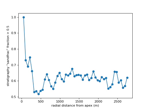
In this example, we explore the sedimentograph [1]. The sedimentograph is a measure of sand fraction of delta stratigraphy. In this implementation, a series of concentric CircularSection are drawn with increasing radius, so the sedimentograph is a function of space.
First, a simple example of computing the sedimentograph, using the compute_sedimentograph function.
By default, the function will generate two bins for the data input for the sediment_volume argument, with the bin divider in the data-range midpoint (i.e., 0.5 for sandfrac data).
# set up the data source
golfcube = dm.sample_data.golf()
golfstrat = dm.cube.StratigraphyCube.from_DataCube(golfcube, dz=0.05)

background = (golfstrat.Z < np.min(golfcube['eta'].data, axis=0))
frozen_sand = golfstrat.export_frozen_variable('sandfrac')

(sedimentograph,
    section_radii,
    sediment_bins) = dm.strat.compute_sedimentograph(
    frozen_sand,
    num_sections=50,
    last_section_radius=2750,
    background=background,
    origin_idx=[golfcube.meta['L0'], golfcube.meta['CTR']])

fig, ax = plt.subplots()
ax.plot(
    section_radii,
    sedimentograph[:, 1],  # plot only the second bin (sandfrac > 0.5)
    'o-')
ax.set_xlabel('radial distance from apex (m)')
ax.set_ylabel('stratigraphy "sandfrac" fraction > 0.5')
plt.show()
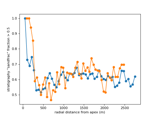
We can mask a portion of the domain, and compute the sedimentograph over just a portion of the domain. The result is a (only slightly) different sedimentograph.
GM = dm.mask.GeometricMask(
    golfcube['eta'][-1],
    angular=dict(
        theta1=np.pi/8,
        theta2=np.pi/2-(np.pi/8))
    )
GM_mask_strat = np.tile(GM.mask, (golfstrat.shape[0], 1, 1))  # a mask with same dimensions as stratigraphy
frozen_sand_mask = frozen_sand.where(GM_mask_strat, np.nan)

(sedimentograph2,
    section_radii2,
    sediment_bins2) = dm.strat.compute_sedimentograph(
    frozen_sand_mask,
    num_sections=50,
    # last_section_radius=2750,
    sediment_bins=None,
    background=background,
    origin_idx=[3, 100])

# add this line to the same plot as above
ax.plot(
    section_radii2,
    sedimentograph2[:, 1],  # plot only the second bin (sandfrac > 0.5)
    'o-')
plt.show()

Using the sedimentograph to evaluate time distribution in subsurface
time_bins = np.linspace(0, golfcube.t[-1], num=7)
(time_sedimentograph,
    time_radii,
    _) = dm.strat.compute_sedimentograph(
    golfstrat['time'],
    num_sections=50,
    last_section_radius=2750,
    sediment_bins=time_bins,
    background=background,
    origin_idx=[3, 100])

import matplotlib
cmap = matplotlib.colormaps['viridis'].resampled(6)
cycler = matplotlib.cycler('color', cmap.colors)
fig, ax = plt.subplots()
ax.set_prop_cycle(cycler)
lines = ax.plot(
    time_radii,
    time_sedimentograph,
    'o-')
ax.set_ylim(0, 1)
time_bin_labels = [f"{time_bins[b]/1e6:.1f}--{time_bins[b+1]/1e6:.1f} million seconds" for b in np.arange(len(time_bins)-1)]
ax.legend(lines, time_bin_labels)
ax.set_xlabel('radial distance from apex (m)')
ax.set_ylabel('stratigraphy fraction in time bin')
plt.show()