Introduction to Section objects

Section lexicon

The Section module defines some terms that are used throughout the code and rest of the documentation.

Most importantly, a Section is defined by a set of coordinates in the dim1-dim2 plane of a Cube.

Note

For advanced use cases, it is possible to create a Section into a Mask, Planform or any array-like data. For this guide, it will be helpful to focus on sections as they cut into a Cube.

Therefore, we transform variable definitions when extracting the Section, and the coordinate system of the section is defined by the along-section direction \(s\) and a vertical section coordinate, which is \(z\) when viewing stratigraphy, and \(t\) when viewing a spacetime section.

The data that make up the section can view the section as a spacetime section by simply calling a variable from the a section into a DataCube.

>>> rcm8cube = dm.sample_data.golf()
>>> strike = dm.section.StrikeSection(rcm8cube, distance_idx=10)
>>> strike['velocity']
<xarray.DataArray 'velocity' (time: 101, s: 200)>
array([[0.2   , 0.2   , 0.2   , ..., 0.2   , 0.2   , 0.2   ],
       [0.    , 0.    , 0.    , ..., 0.    , 0.    , 0.    ],
       [0.    , 0.0025, 0.    , ..., 0.    , 0.    , 0.    ],
       ...,
       [0.    , 0.    , 0.    , ..., 0.0025, 0.    , 0.    ],
       [0.    , 0.    , 0.    , ..., 0.    , 0.    , 0.    ],
       [0.    , 0.    , 0.    , ..., 0.0025, 0.    , 0.    ]],
      dtype=float32)
Coordinates:
  * s        (s) float64 0.0 50.0 100.0 150.0 ... 9.85e+03 9.9e+03 9.95e+03
  * time     (time) float32 0.0 5e+05 1e+06 1.5e+06 ... 4.9e+07 4.95e+07 5e+07
Attributes:
    slicetype:           data_section
    knows_stratigraphy:  False
    knows_spacetime:     True

If a DataCube has preservation information (i.e., if the stratigraphy_from() method has been called), then the xarray object that is returned has this information too. The same spacetime data can be requested in the “preserved” form, where non-preserved t-x-y points are masked with np.nan.

>>> rcm8cube.stratigraphy_from('eta')
>>> strike['velocity'].strat.as_preserved()
<xarray.DataArray 'velocity' (time: 101, s: 200)>
array([[0.2, 0.2, 0.2, ..., 0.2, 0.2, 0.2],
       [nan, nan, nan, ..., nan, nan, nan],
       [nan, nan, nan, ..., nan, nan, nan],
       ...,
       [nan, nan, nan, ..., nan, nan, nan],
       [nan, nan, nan, ..., nan, nan, nan],
       [nan, nan, nan, ..., nan, nan, nan]], dtype=float32)
Coordinates:
  * s        (s) float64 0.0 50.0 100.0 150.0 ... 9.85e+03 9.9e+03 9.95e+03
  * time     (time) float32 0.0 5e+05 1e+06 1.5e+06 ... 4.9e+07 4.95e+07 5e+07
Attributes:
    slicetype:           data_section
    knows_stratigraphy:  True
    knows_spacetime:     True

Note

The section has access to the preservation information of the data, even though it was instantiated prior to the computation of preservation!

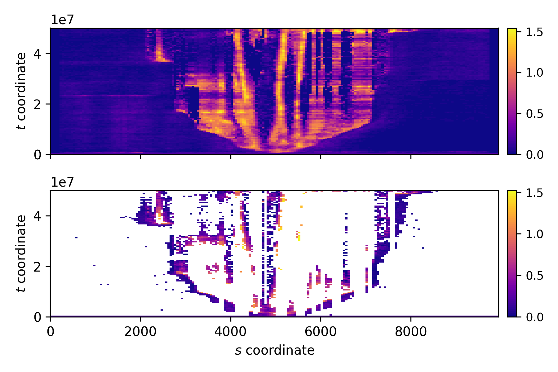
We can display the arrays using matplotlib to examine the spatiotemporal change of any variable; show the velocity in the below examples.

>>> fig, ax = plt.subplots(2, 1, sharex=True, figsize=(6, 3.5))
>>> golfcube.sections['demo'].show('velocity', ax=ax[0])
>>> ax[0].set_ylabel('$t$ coordinate')

>>> golfcube.sections['demo'].show('velocity', data='preserved', ax=ax[1])
>>> ax[1].set_ylabel('$t$ coordinate')

>>> ax[1].set_xlabel('$s$ coordinate')

(png, hires.png)

Note that in this visual all non-preserved spacetime points have been masked and are shown as white. See the numpy MaskedArray documentation for more information on interacting with masked arrays.

Creating sections into other data types

You can also create Sections into an object other than a Cube, such as a Mask or Planform or arbitrary data.

See the example here for several examples.