Introduction to Planform objects

Multiple definitions of the delta planform are supported. These planform objects can be used as starting points for binary mask computation. If not specified explicitly, they are often implicitly part of binary mask creation.

Below we demonstrate instantiation of both the OpeningAnglePlanform and the MorphologicalPlanform objects.

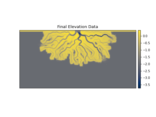
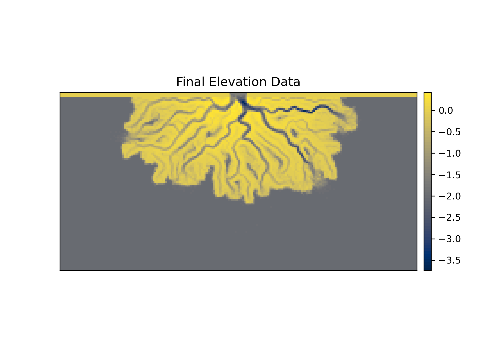
For each we start with the same example dataset, and use the elevation data at the end of the simulation.

golfcube = dm.sample_data.golf()

fig, ax = plt.subplots()
golfcube.quick_show('eta', idx=-1, ax=ax)
ax.set_title('Final Elevation Data')
plt.show()

(png, hires.png)

The OpeningAnglePlanform

This planform object is based around the Opening Angle Method [1].

The OpeningAnglePlanform can be created directly from elevation data:

golfcube = dm.sample_data.golf()
OAP = dm.plan.OpeningAnglePlanform.from_elevation_data(
  golfcube['eta'][-1, :, :], elevation_threshold=0)

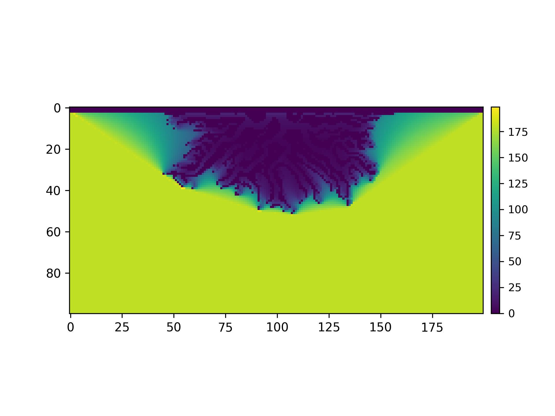
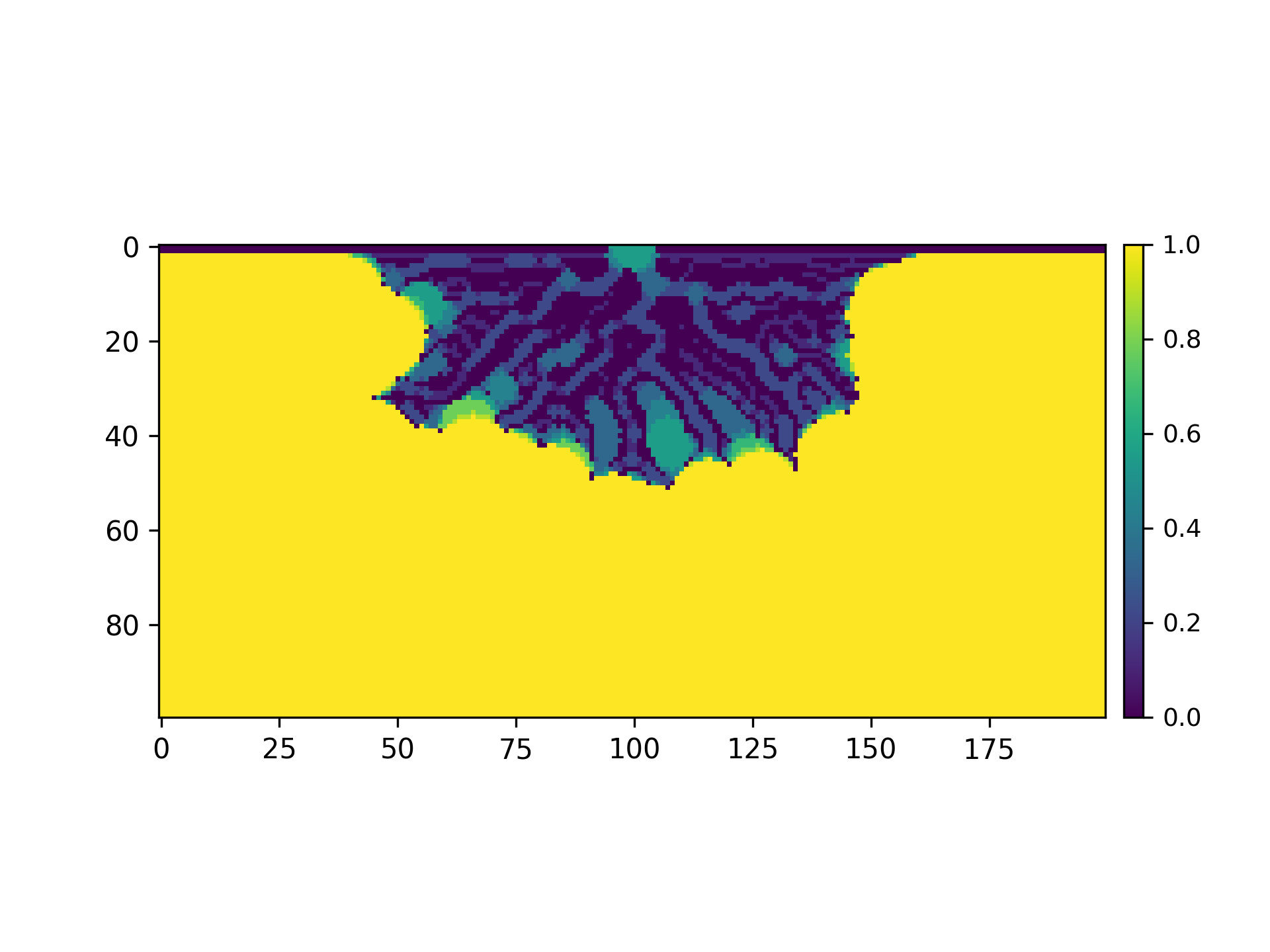
All planforms have a composite_array attribute from which a contour is extracted when defining the shoreline. In the case of the OpeningAnglePlanform, the composite_array is the “sea angles” array from the Opening Angle Method.

fig, ax = plt.subplots()
im = ax.imshow(OAP.composite_array)
dm.plot.append_colorbar(im, ax=ax)
plt.show()

(png, hires.png)

[1]

Shaw, J. B., Wolinsky, M. A., Paola, C., & Voller, V. R. (2008). An image‐based method for shoreline mapping on complex coasts. Geophysical Research Letters, 35(12).

The MorphologicalPlanform

This planform object uses mathematical morphology to identify the delta planform, inspired by Geleynse et al (2012) [2].

The MorphologicalPlanform can also be created directly from elevation data:

MP = dm.plan.MorphologicalPlanform.from_elevation_data(
  golfcube['eta'][-1, :, :], elevation_threshold=0, max_disk=8)

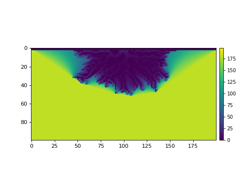
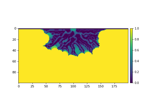
In this case, the composite_array attribute of the planform represents the inverse of the average pixel value when different sized disks are used to perform the binary closing on the elevation data.

fig, ax = plt.subplots()
im = ax.imshow(MP.composite_array)
dm.plot.append_colorbar(im, ax=ax)
plt.show()

(png, hires.png)

[2]

Geleynse, N., Voller, V. R., Paola, C., & Ganti, V. (2012). Characterization of river delta shorelines. Geophysical research letters, 39(17).

Mask Extraction

These planform objects can be used to extract shoreline masks as well as land masks. The masking API accepts either planform object as an input, making it easy to swap one planform for the other in a masking workflow.

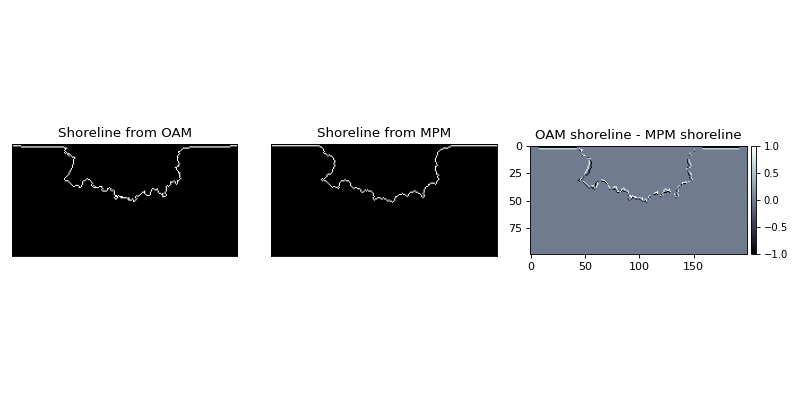
As an example, we will extract a shoreline from both planforms shown above. Of course the two methods are different, so the shorelines identified will also be different.

SM_from_OAM = dm.mask.ShorelineMask.from_Planform(
  OAP, contour_threshold=75)

SM_from_MPM = dm.mask.ShorelineMask.from_Planform(
  MP, contour_threshold=0.75)

fig, ax = plt.subplots(1, 3, figsize=(10, 5))

SM_from_OAM.show(ax=ax[0])
ax[0].set_title('Shoreline from OAM')

SM_from_MPM.show(ax=ax[1])
ax[1].set_title('Shoreline from MPM')

diff_im = ax[2].imshow(
  SM_from_OAM.mask.astype(float) - SM_from_MPM.mask.astype(float),
  interpolation=None, cmap='bone')
ax[2].set_title('OAM shoreline - MPM shoreline')
dm.plot.append_colorbar(diff_im, ax=ax[2])

plt.tight_layout()
plt.show()

(png, hires.png)

Both methods require the user to set a “contour threshold” value when extracting the shoreline. The shoreline ends up being a contour extracted at this value from the planform composite_array.

The OAM method is relatively insensitive to the value of this threshold, whereas the MPM method can be more sensitive, depending on the range of disk sizes used. Overall though, this example shows that the two methods produce roughly similar shorelines, and the syntax of the function calls to produce the planforms and the shoreline masks is more similar than it is different.