Introduction to Masking objects

Note

Need description of what masks are conceptually (a binary classification of some field), and what they are in practice (an object that wraps an array that indicates True and False).

Computing masks efficiently

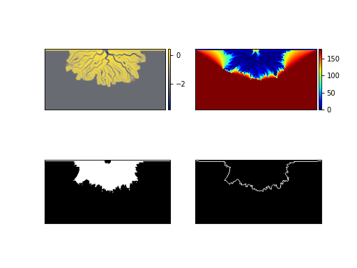
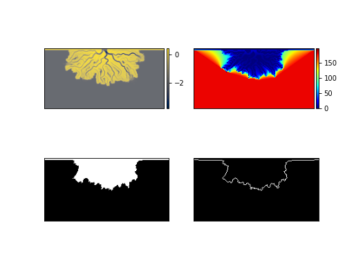
If you are creating multiple masks for the same planform data (e.g., for the same time slice of data for the physical domain), it is computationally advantageous to create a single OpeningAnglePlanform, and use this OAP to create other masks.

For example:

>>> golfcube = dm.sample_data.golf()

>>> OAP = dm.plan.OpeningAnglePlanform.from_elevation_data(
...     golfcube['eta'][-1, :, :],
...     elevation_threshold=0)

>>> lm = dm.mask.LandMask.from_Planform(OAP)
>>> sm = dm.mask.ShorelineMask.from_Planform(OAP)

>>> fig, ax = plt.subplots(2, 2)
>>> golfcube.quick_show('eta', idx=-1, ax=ax[0, 0])
>>> OAP.show(ax=ax[0, 1])
>>> lm.show(ax=ax[1, 0])
>>> sm.show(ax=ax[1, 1])

(png, hires.png)

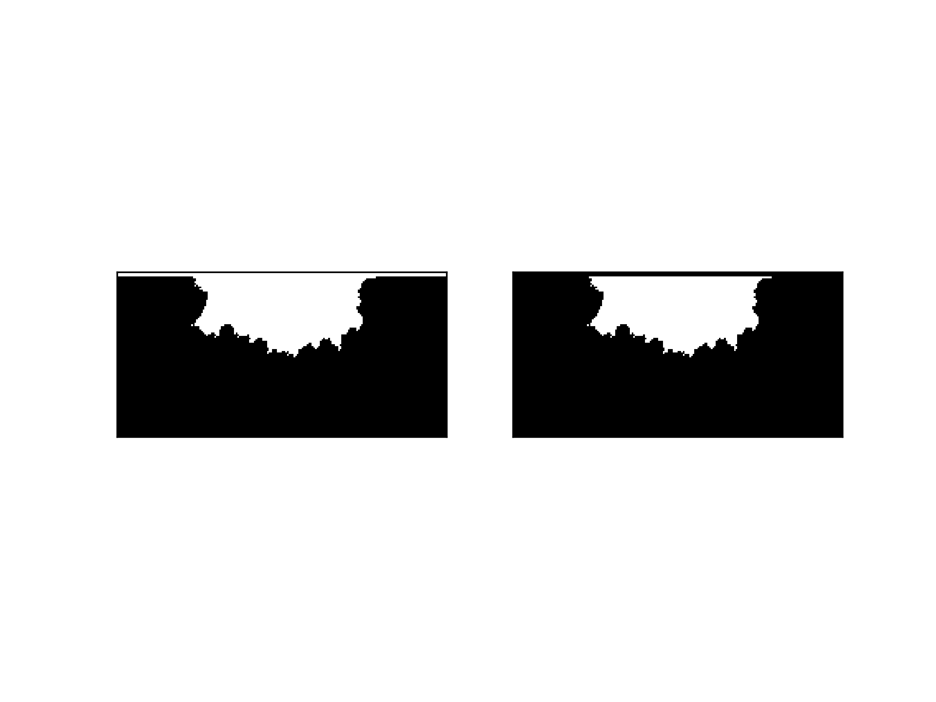
Trimming masks before input

Sometimes it is helpful to trim a mask, essentially replacing values with a different value, before using the mask for analysis or input to functions.

>>> golfcube = dm.sample_data.golf()

>>> m0 = dm.mask.LandMask(
...     golfcube['eta'][-1, :, :],
...     elevation_threshold=0)
>>> m1 = dm.mask.LandMask(
...     golfcube['eta'][-1, :, :],
...     elevation_threshold=0)

>>> # trim one of the masks
>>> m1.trim_mask(length=3)

>>> fig, ax = plt.subplots(1, 2)
>>> m0.show(ax=ax[0])
>>> m1.show(ax=ax[1])
>>> plt.show()

(png, hires.png)